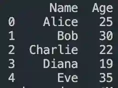
#dataframe indexing

[codewithnazam]

DataFrame in Pandas: Guide to Creating Awesome DataFrames

Explore how to create a dataframe in Pandas, including data input methods, customization options, and practical examples.

Data analysis used to be a daunting task, reserved for statisticians and mathematicians. But with the rise of powerful tools like Python and its fantastic library, Pandas, anyone can become a data whiz! Pandas, in particular, shines with its DataFrames, these nifty tables that organize and manipulate data like magic. But where do you start? Fear not, fellow data enthusiast, for this guide will…

[lighthouseteck]

Lasso Regression Analysis

import numpy as np

import pandas as pd

import matplotlib.pyplot as plt

from sklearn.linear_model import LassoCV, Lasso

from sklearn.model_selection import KFold, train_test_split

from sklearn.metrics import mean_squared_error, r2_score

from sklearn.preprocessing import StandardScaler

import seaborn as sns

# Set random seed for reproducibility

np.random.seed(42)

# 1. Generate some sample data (replace with your own data)

def generate_sample_data(n_samples=200, n_features=50, n_informative=10):

    """

    Generate synthetic data with only some informative features.

    - n_samples: Number of data points

    - n_features: Total number of predictor variables

    - n_informative: Number of predictors that actually affect the response

    """

    # Generate predictor variables X

    X = np.random.normal(size=(n_samples, n_features))

    # Generate the response variable y based on only n_informative predictors

    # Add some random noise as well

    true_coef = np.zeros(n_features)

    true_coef[:n_informative] = np.random.uniform(low=0.5, high=3.0, size=n_informative) * np.random.choice([-1, 1], size=n_informative)

    y = np.dot(X, true_coef) + np.random.normal(scale=0.5, size=n_samples)

    # Create feature names

    feature_names = [f'feature_{i}' for i in range(n_features)]

    # Convert to DataFrame for better handling

    df = pd.DataFrame(X, columns=feature_names)

    df['target'] = y

    return df, true_coef, feature_names

# Generate data

df, true_coef, feature_names = generate_sample_data(n_samples=200, n_features=50, n_informative=10)

# Split data into training and testing sets

X = df.drop('target', axis=1)

y = df['target']

X_train, X_test, y_train, y_test = train_test_split(X, y, test_size=0.2, random_state=42)

# 2. Standardize features (important for LASSO)

scaler = StandardScaler()

X_train_scaled = scaler.fit_transform(X_train)

X_test_scaled = scaler.transform(X_test)

# 3. Set up LASSO with k-fold cross validation

# We'll use LassoCV which automatically finds the best alpha parameter

k_folds = 5

kf = KFold(n_splits=k_folds, shuffle=True, random_state=42)

# Set up a range of alpha values to try

alphas = np.logspace(-4, 1, 50)

# Initialize LassoCV

lasso_cv = LassoCV(

    alphas=alphas,

    cv=kf,

    max_iter=10000,

    tol=0.0001,

    n_jobs=-1  # Use all available cores

)

# Fit the model

lasso_cv.fit(X_train_scaled, y_train)

# 4. Get the best alpha value

best_alpha = lasso_cv.alpha_

print(f"Best alpha (regularization parameter): {best_alpha:.6f}")

# 5. Build final LASSO model using the best alpha

lasso_model = Lasso(alpha=best_alpha)

lasso_model.fit(X_train_scaled, y_train)

# 6. Evaluate the model

y_pred_train = lasso_model.predict(X_train_scaled)

y_pred_test = lasso_model.predict(X_test_scaled)

train_r2 = r2_score(y_train, y_pred_train)

test_r2 = r2_score(y_test, y_pred_test)

train_mse = mean_squared_error(y_train, y_pred_train)

test_mse = mean_squared_error(y_test, y_pred_test)

print(f"Training R²: {train_r2:.4f}")

print(f"Testing R²: {test_r2:.4f}")

print(f"Training MSE: {train_mse:.4f}")

print(f"Testing MSE: {test_mse:.4f}")

# 7. Identify selected features

coef = pd.Series(lasso_model.coef_, index=X.columns)

selected_features = coef[coef != 0].index.tolist()

n_selected = len(selected_features)

print(f"\nNumber of features selected by LASSO: {n_selected} out of {len(X.columns)}")

print("\nSelected features and their coefficients:")

selected_coef = coef[selected_features].sort_values(ascending=False)

for feature, value in selected_coef.items():

    print(f"{feature}: {value:.6f}")

# 8. Visualize feature coefficients

plt.figure(figsize=(14, 6))

sns.barplot(x=selected_coef.index, y=selected_coef.values)

plt.xticks(rotation=90)

plt.title('LASSO Selected Features and Their Coefficients')

plt.tight_layout()

plt.show()

# 9. Visualize LASSO path (how coefficients change with alpha)

# This helps understand how variables are selected

plt.figure(figsize=(14, 6))

alphas_to_plot = np.logspace(-4, 0, 100)

coefs = []

for alpha in alphas_to_plot:

    lasso = Lasso(alpha=alpha)

    lasso.fit(X_train_scaled, y_train)

    coefs.append(lasso.coef_)

ax = plt.gca()

ax.plot(np.log10(alphas_to_plot), np.array(coefs))

ax.set_xlabel('log(alpha)')

ax.set_ylabel('Coefficients')

ax.set_title('LASSO Path: Coefficient Values vs Regularization Strength')

ax.axvline(np.log10(best_alpha), color='k', linestyle='--', label=f'Best alpha: {best_alpha:.6f}')

ax.legend()

plt.tight_layout()

plt.show()

# 10. Compare actual vs predicted coefficients

# For synthetic data only - skip this part if using real data

if 'true_coef' in locals():

    # Plot actual vs predicted coefficients

    plt.figure(figsize=(12, 6))

    plt.scatter(range(len(true_coef)), true_coef, alpha=0.7, label='True coefficients')

    plt.scatter(range(len(lasso_model.coef_)), lasso_model.coef_, alpha=0.7, label='LASSO coefficients')

    plt.xlabel('Feature index')

    plt.ylabel('Coefficient value')

    plt.legend()

    plt.title('True Coefficients vs LASSO Coefficients')

    plt.tight_layout()

    plt.show()

    # Calculate the number of correctly identified informative features

    true_informative = np.where(true_coef != 0)[0]

    selected_indices = np.where(lasso_model.coef_ != 0)[0]

    correctly_identified = np.intersect1d(true_informative, selected_indices)

    print(f"\nOut of {len(true_informative)} truly informative features, LASSO correctly identified {len(correctly_identified)}")

    print(f"False positives: {len(selected_indices) - len(correctly_identified)}")

    print(f"False negatives: {len(true_informative) - len(correctly_identified)}")

# 11. Function to apply the model to new data

def predict_with_lasso(new_data, scaler, lasso_model):

    """

    Make predictions using the fitted LASSO model

    Parameters:

    -----------

    new_data : DataFrame

        New data to predict (same features as training data)

    scaler : StandardScaler

        Fitted scaler object

    lasso_model : Lasso

        Fitted LASSO model

    Returns:

    --------

    predictions : array

        Predicted target values

    """

    # Scale the new data

    new_data_scaled = scaler.transform(new_data)

    # Make predictions

    predictions = lasso_model.predict(new_data_scaled)

    return predictions

# Example: Generate some new data and make predictions

# In real applications, this would be your new data

new_data_example = pd.DataFrame(np.random.normal(size=(5, len(X.columns))), columns=X.columns)

predictions = predict_with_lasso(new_data_example, scaler, lasso_model)

print("\nPredictions for new data:")

print(predictions)

[gregtechdotpy]

5/12/2025

Today I got hooked on the idea of taking the Gregtech New Horizons modpack for Minecraft and making a program that would combine a lot of different necessary calculators into it. Online I found a spreadsheet (https://docs.google.com/spreadsheets/d/1HgrUWh39L4zA4QDWOSHOovPek1s1eAK1VsZQy_D0zjQ/edit#gid=962322443) that helped with balancing how many coke ovens to water to boilers you need for steam production (something that involves an unnecessary amount of variables, but welcome to GTNH), and decided that I wanted to convert it as my first bite, along with a calculator for how many blocks I would need to build different tank sizes. Eventually I want to move it to a website, but for now it is hosted on my GitHub (https://github.com/lokon100/greghell) while I am starting it!

I haven’t worked in Python for a bit so it was great to come back to it and look at it with fresh eyes, especially for how I stored my variables! I stored my static variables in Pandas Series and Dataframes, which kept it pretty neat and organized.

The “new thing” I decided to look into was how to streamline having a user choose something from a list, and after some searching around I landed on this solution from StackOverflow (https://stackoverflow.com/questions/37565793/how-to-let-the-user-select-an-input-from-a-finite-list) that shows how to have a user choose from a dictionary index. I modified the code so that it would work from a list instead of an index, and it worked perfectly for inputting variables at the beginning of a run!

def selectFromList(options, name="option"):     index = 0     print('Select a ' + name + ':')     for optionName in options:         index = index + 1         print(str(index) + ') ' + optionName)     inputValid = False     while not inputValid:         inputRaw = input(name + ': ')         inputNo = int(inputRaw) - 1         if inputNo > -1 and inputNo < len(options):             selected = options[inputNo]             break         else:             print('Please select a valid ' + name + ' number')     return selected

Rereading my code a bit after I finished it I realized that not very much is different between the two “pressure types” of boilers, and I actually managed to knock a chunk of it off to streamline it which always feels pretty nice! Note to self- always check whether the only difference between your functions is one variable, because you can always just feed those in versus writing out a whole second function and using if loops!

I also noticed that three of the variables would probably never change, so I commented out the input lines and put in static values so that I could have ease of using it for now, but when I finish and publish the sets of calculators I can make it so that everyone can adjust it.

def boiler_math(pressure):     boilerSize = uf.selectFromList(boilerVars['Shape'].tolist())     timeFrame = uf.selectFromList(timeTicks.index.to_list())     fuelType = uf.selectFromList(ovenProd.index.to_list())     numBoilers = int(input("How many boilers?"))     numWater = int(input("How many water tanks?"))     numOvens = int(input("How many coke ovens?"))     rainMod = float(input("What is the rain modifier?"))     if pressure == "high":         solidWater, solidSteam, waterProd = boiler_high(boilerSize, timeFrame, fuelType, numBoilers, numWater, numOvens,rainMod)         liquidWater, liquidSteam, waterProd = boiler_high(boilerSize, timeFrame, 'creosote', numBoilers, numWater, numOvens,rainMod)         totalWater = waterProd-(solidWater+liquidWater)         totalSteam = solidSteam+liquidSteam         print("Total Water Difference: " + str(totalWater) + " Total Steam Production: " + str(totalSteam))     if pressure == "low":         solidWater, solidSteam, waterProd = boiler_low(boilerSize, timeFrame, fuelType, numBoilers, numWater, numOvens,rainMod)         liquidWater, liquidSteam, waterProd = boiler_low(boilerSize, timeFrame, 'creosote', numBoilers, numWater, numOvens,rainMod)         totalWater = waterProd-(solidWater+liquidWater)         totalSteam = solidSteam+liquidSteam         print("Total Water Difference: " + str(totalWater) + " Total Steam Production: " + str(totalSteam)) def boiler_low(boilerSize, timeFrame, fuelType, numBoilers, numWater, numOvens, rainMod):     tanks = boilerVars.loc[boilerVars['Shape'] == boilerSize, 'Size'].iloc[0]     lpMod = boilerVars.loc[boilerVars['Shape'] == boilerSize, 'LP'].iloc[0]     numTicks = timeTicks.loc[timeFrame]     burnTime = fuelTimes.loc[fuelType]     fuelConsumption = lpMod*numTicks/burnTime*numBoilers     steamProduction = tanks*numTicks*10*numBoilers     waterConsumption = steamProduction/150     ovenProduction = ovenProd.loc[fuelType]*numTicks*numOvens     waterProduction = numWater*rainMod*1.25*numTicks     fuelDifference = ovenProduction-fuelConsumption     waterDifference = waterProduction-waterConsumption     print("For " + fuelType + " use")     print("Fuel Difference: " + str(fuelDifference) + " Water Difference: " + str(waterDifference) + " Steam Production: " + str(steamProduction))     return waterConsumption, steamProduction, waterProduction def boiler_high(boilerSize, timeFrame, fuelType, numBoilers, numWater, numOvens, rainMod):     tanks = boilerVars.loc[boilerVars['Shape'] == boilerSize, 'Size'].iloc[0]     hpMod = boilerVars.loc[boilerVars['Shape'] == boilerSize, 'HP'].iloc[0]     numTicks = timeTicks.loc[timeFrame]     burnTime = fuelTimes.loc[fuelType]     fuelConsumption = hpMod*numTicks/burnTime*numBoilers     steamProduction = tanks*numTicks*10*numBoilers     waterConsumption = steamProduction/150     ovenProduction = ovenProd.loc[fuelType]*numTicks*numOvens     waterProduction = numWater*rainMod*1.25*numTicks     fuelDifference = ovenProduction-fuelConsumption     waterDifference = waterProduction-waterConsumption     print("For " + fuelType + " use")     print("Fuel Difference: " + str(fuelDifference) + " Water Difference: " + str(waterDifference) + " Steam Production: " + str(steamProduction))     return waterConsumption, steamProduction, waterProduction

Vs

def boiler_math():     pressure = uf.selectFromList(["LP", "HP"])     boilerSize = uf.selectFromList(boilerVars['Shape'].tolist())     timeFrame = "hour"                                              #uf.selectFromList(timeTicks.index.to_list())     fuelType = uf.selectFromList(ovenProd.index.to_list())     numBoilers = 1                                                  #int(input("How many boilers?"))     numWater = int(input("How many water tanks?"))     numOvens = int(input("How many coke ovens?"))     rainMod = 0.8                                                   #float(input("What is the rain modifier?"))     solidWater, solidSteam, waterProd = boiler_vars(boilerSize, timeFrame, fuelType, numBoilers, numWater, numOvens,rainMod, pressure)     liquidWater, liquidSteam, waterProd = boiler_vars(boilerSize, timeFrame, 'creosote', numBoilers, numWater, numOvens,rainMod, pressure)     totalWater = waterProd-(solidWater+liquidWater)     totalSteam = solidSteam+liquidSteam     print("Total Water Difference: " + str(totalWater) + " Total Steam Production: " + str(totalSteam)) def boiler_vars(boilerSize, timeFrame, fuelType, numBoilers, numWater, numOvens, rainMod, pressure):     tanks = boilerVars.loc[boilerVars['Shape'] == boilerSize, 'Size'].iloc[0]     lpMod = boilerVars.loc[boilerVars['Shape'] == boilerSize, pressure].iloc[0]     numTicks = timeTicks.loc[timeFrame]     burnTime = fuelTimes.loc[fuelType]     fuelConsumption = lpMod*numTicks/burnTime*numBoilers     steamProduction = tanks*numTicks*10*numBoilers     waterConsumption = steamProduction/150     ovenProduction = ovenProd.loc[fuelType]*numTicks*numOvens     waterProduction = numWater*rainMod*1.25*numTicks     fuelDifference = ovenProduction-fuelConsumption     waterDifference = waterProduction-waterConsumption     print("For " + fuelType + " use")     print("Fuel Difference: " + str(fuelDifference) + " Water Difference: " + str(waterDifference) + " Steam Production: " + str(steamProduction))     return waterConsumption, steamProduction, waterProduction

[b4kingg]

Analyzing the Relationship Between Education Level and Political Affiliation: A Chi-Square Test of Independence

In this project, I explored whether there is a significant association between education level and political affiliation using the Chi-Square Test of Independence. This statistical approach is ideal for examining relationships between categorical variables.

Research Question

Is there a significant association between a person's education level and their political affiliation?

Methodology

I used Python with the scipy.stats, pandas, and matplotlib libraries to conduct the analysis. The dataset contains information about individuals' education levels (categorized as "High School," "College," and "Graduate") and their political affiliations (categorized as "Liberal," "Moderate," and "Conservative").

Python Code

import numpy as np import pandas as pd import matplotlib.pyplot as plt from scipy.stats import chi2_contingency import seaborn as sns

#Create a sample dataset (in a real scenario, you would import your data)

data = { 'Education': ['High School', 'High School', 'High School', 'High School', 'High School', 'College', 'College', 'College', 'College', 'College', 'Graduate', 'Graduate', 'Graduate', 'Graduate', 'Graduate', 'High School', 'High School', 'College', 'College', 'Graduate', 'Graduate', 'Graduate', 'High School', 'College', 'College', 'Graduate', 'High School', 'High School', 'College', 'Graduate'], 'Political_Affiliation': ['Conservative', 'Conservative', 'Conservative', 'Moderate', 'Liberal', 'Conservative', 'Conservative', 'Moderate', 'Moderate', 'Liberal', 'Conservative', 'Moderate', 'Liberal', 'Liberal', 'Liberal', 'Conservative', 'Moderate', 'Moderate', 'Liberal', 'Moderate', 'Liberal', 'Liberal', 'Conservative', 'Conservative', 'Liberal', 'Liberal', 'Conservative', 'Moderate', 'Liberal', 'Liberal'] }

#Create DataFrame

df = pd.DataFrame(data)

#Create a contingency table

contingency_table = pd.crosstab(df['Education'], df['Political_Affiliation']) print("Contingency Table:") print(contingency_table)

#Perform Chi-Square Test of Independence

chi2, p, dof, expected = chi2_contingency(contingency_table)

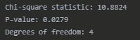
print("\nChi-Square Test Results:") print(f"Chi-square statistic: {chi2:.4f}") print(f"P-value: {p:.4f}") print(f"Degrees of freedom: {dof}")

#Visualize the contingency table

plt.figure(figsize=(10, 6)) sns.heatmap(contingency_table, annot=True, fmt='d', cmap='Blues') plt.title('Contingency Table: Education Level vs. Political Affiliation') plt.xlabel('Political Affiliation') plt.ylabel('Education Level') plt.tight_layout() plt.savefig('chi_square_heatmap.png')

#If the Chi-Square test is significant and we have more than 2 categories,

#we need to perform post-hoc analysis

if p < 0.05 and contingency_table.shape[0] > 2 and contingency_table.shape[1] > 2: print("\nPost-hoc Analysis:") # Calculate the standardized residuals observed = contingency_table.values row_totals = observed.sum(axis=1) col_totals = observed.sum(axis=0) total = observed.sum()expected_array = np.outer(row_totals, col_totals) / total residuals = (observed - expected_array) / np.sqrt(expected_array) # Create a DataFrame for residuals residuals_df = pd.DataFrame( residuals, index=contingency_table.index, columns=contingency_table.columns ) print("\nStandardized Residuals:") print(residuals_df) # Interpret residuals print("\nCell-by-cell interpretation:") for i, education in enumerate(contingency_table.index): for j, affiliation in enumerate(contingency_table.columns): residual = residuals[i, j] if abs(residual) > 1.96: # Using 95% confidence level relationship = "more" if residual > 0 else "fewer" print(f"There are significantly {relationship} {education} individuals with {affiliation} affiliation than expected by chance (residual = {residual:.2f}).")

Results

Contingency Table:

Chi-Square Test Results:

Post-hoc Analysis:

Interpretation

The Chi-Square Test of Independence yielded a statistic of 10.88 with a p-value of 0.0279, which is less than our significance level of 0.05. Therefore, we reject the null hypothesis and conclude that there is a significant association between education level and political affiliation.

The post-hoc analysis reveals specific patterns in this relationship:

People with a Graduate education are significantly less likely to identify as Conservative and more likely to identify as Liberal than would be expected by chance.

People with a High School education are significantly more likely to identify as Conservative and less likely to identify as Liberal than would be expected by chance.

The College education group does not show any significant deviations from expected frequencies in any political affiliation category.

These findings suggest that education level may influence political ideology, with higher education levels correlating with more liberal views. However, it's important to note that correlation does not imply causation, and other factors not examined in this analysis might also contribute to this relationship.

Conclusion

This Chi-Square Test of Independence demonstrates a statistically significant relationship between education level and political affiliation. The analysis highlights how the proportions of political affiliations differ across education levels, with notable patterns emerging particularly among those with Graduate and High School education.

Heatmap Description:

The heatmap displays a 3x3 grid showing the frequency counts for each combination of education level (rows) and political affiliation (columns).

College row: Conservative (3), Liberal (5), Moderate (4)

Graduate row: Conservative (1), Liberal (8), Moderate (2)

High School row: Conservative (6), Liberal (1), Moderate (2)

Higher frequency cells appear in darker blue colors.

The highest frequency (8) is for Graduate-Liberal, shown as the darkest cell.

The lowest frequency (1) is for Graduate-Conservative and High School-Liberal, shown as the lightest cells.

[fromdevcom]

Pandas DataFrame Tutorial: Ways to Create and Manipulate Data in Python Are you diving into data analysis with Python? Then you're about to become best friends with pandas DataFrames. These powerful, table-like structures are the backbone of data manipulation in Python, and knowing how to create them is your first step toward becoming a data analysis expert. In this comprehensive guide, we'll explore everything you need to know about creating pandas DataFrames, from basic methods to advanced techniques. Whether you're a beginner or looking to level up your skills, this tutorial has got you covered. Getting Started with Pandas Before we dive in, let's make sure you have everything set up. First, you'll need to install pandas if you haven't already: pythonCopypip install pandas Then, import pandas in your Python script: pythonCopyimport pandas as pd 1. Creating a DataFrame from Lists The simplest way to create a DataFrame is using Python lists. Here's how: pythonCopy# Creating a basic DataFrame from lists data = 'name': ['John', 'Emma', 'Alex', 'Sarah'], 'age': [28, 24, 32, 27], 'city': ['New York', 'London', 'Paris', 'Tokyo'] df = pd.DataFrame(data) print(df) This creates a clean, organized table with your data. The keys in your dictionary become column names, and the values become the data in each column. 2. Creating a DataFrame from NumPy Arrays When working with numerical data, NumPy arrays are your friends: pythonCopyimport numpy as np # Creating a DataFrame from a NumPy array array_data = np.random.rand(4, 3) df_numpy = pd.DataFrame(array_data, columns=['A', 'B', 'C'], index=['Row1', 'Row2', 'Row3', 'Row4']) print(df_numpy) 3. Reading Data from External Sources Real-world data often comes from files. Here's how to create DataFrames from different file formats: pythonCopy# CSV files df_csv = pd.read_csv('your_file.csv') # Excel files df_excel = pd.read_excel('your_file.xlsx') # JSON files df_json = pd.read_json('your_file.json') 4. Creating a DataFrame from a List of Dictionaries Sometimes your data comes as a list of dictionaries, especially when working with APIs: pythonCopy# List of dictionaries records = [ 'name': 'John', 'age': 28, 'department': 'IT', 'name': 'Emma', 'age': 24, 'department': 'HR', 'name': 'Alex', 'age': 32, 'department': 'Finance' ] df_records = pd.DataFrame(records) print(df_records) 5. Creating an Empty DataFrame Sometimes you need to start with an empty DataFrame and fill it later: pythonCopy# Create an empty DataFrame with defined columns columns = ['Name', 'Age', 'City'] df_empty = pd.DataFrame(columns=columns) # Add data later new_row = 'Name': 'Lisa', 'Age': 29, 'City': 'Berlin' df_empty = df_empty.append(new_row, ignore_index=True) 6. Advanced DataFrame Creation Techniques Using Multi-level Indexes pythonCopy# Creating a DataFrame with multi-level index arrays = [ ['2023', '2023', '2024', '2024'], ['Q1', 'Q2', 'Q1', 'Q2'] ] data = 'Sales': [100, 120, 150, 180] df_multi = pd.DataFrame(data, index=arrays) print(df_multi) Creating Time Series DataFrames pythonCopy# Creating a time series DataFrame dates = pd.date_range('2024-01-01', periods=6, freq='D') df_time = pd.DataFrame(np.random.randn(6, 4), index=dates, columns=['A', 'B', 'C', 'D']) Best Practices and Tips Always Check Your Data Types pythonCopy# Check data types of your DataFrame print(df.dtypes) Set Column Names Appropriately Use clear, descriptive column names without spaces: pythonCopydf.columns = ['first_name', 'last_name', 'email'] Handle Missing Data pythonCopy# Check for missing values print(df.isnull().sum()) # Fill missing values df.fillna(0, inplace=True) Common Pitfalls to Avoid Memory Management: Be cautious with large datasets. Use appropriate data types to minimize memory usage:

pythonCopy# Optimize numeric columns df['integer_column'] = df['integer_column'].astype('int32') Copy vs. View: Understand when you're creating a copy or a view: pythonCopy# Create a true copy df_copy = df.copy() Conclusion Creating pandas DataFrames is a fundamental skill for any data analyst or scientist working with Python. Whether you're working with simple lists, complex APIs, or external files, pandas provides flexible and powerful ways to structure your data. Remember to: Choose the most appropriate method based on your data source Pay attention to data types and memory usage Use clear, consistent naming conventions Handle missing data appropriately With these techniques in your toolkit, you're well-equipped to handle any data manipulation task that comes your way. Practice with different methods and explore the pandas documentation for more advanced features as you continue your data analysis journey. Additional Resources Official pandas documentation Pandas cheat sheet Python for Data Science Handbook Real-world pandas examples on GitHub Now you're ready to start creating and manipulating DataFrames like a pro. Happy coding!

[machinelearningcoursera]

K-mean Analysis

Script:

from pandas import Series, DataFrame import pandas as pd import numpy as np import matplotlib.pylab as plt from sklearn.model_selection import train_test_split from sklearn import preprocessing from sklearn.cluster import KMeans import os """ Data Management """

data = pd.read_csv("tree_addhealth.csv")

upper-case all DataFrame column names

data.columns = map(str.upper, data.columns)

Data Management

data_clean = data.dropna()

subset clustering variables

cluster=data_clean[['ALCEVR1','MAREVER1','ALCPROBS1','DEVIANT1','VIOL1', 'DEP1','ESTEEM1','SCHCONN1','PARACTV', 'PARPRES','FAMCONCT']] cluster.describe()

standardize clustering variables to have mean=0 and sd=1

clustervar=cluster.copy() clustervar['ALCEVR1']=preprocessing.scale(clustervar['ALCEVR1'].astype('float64')) clustervar['ALCPROBS1']=preprocessing.scale(clustervar['ALCPROBS1'].astype('float64')) clustervar['MAREVER1']=preprocessing.scale(clustervar['MAREVER1'].astype('float64')) clustervar['DEP1']=preprocessing.scale(clustervar['DEP1'].astype('float64')) clustervar['ESTEEM1']=preprocessing.scale(clustervar['ESTEEM1'].astype('float64')) clustervar['VIOL1']=preprocessing.scale(clustervar['VIOL1'].astype('float64')) clustervar['DEVIANT1']=preprocessing.scale(clustervar['DEVIANT1'].astype('float64')) clustervar['FAMCONCT']=preprocessing.scale(clustervar['FAMCONCT'].astype('float64')) clustervar['SCHCONN1']=preprocessing.scale(clustervar['SCHCONN1'].astype('float64')) clustervar['PARACTV']=preprocessing.scale(clustervar['PARACTV'].astype('float64')) clustervar['PARPRES']=preprocessing.scale(clustervar['PARPRES'].astype('float64'))

split data into train and test sets

clus_train, clus_test = train_test_split(clustervar, test_size=.3, random_state=123)

k-means cluster analysis for 1-9 clusters

from scipy.spatial.distance import cdist clusters=range(1,9) meandist=[]

for k in clusters: model=KMeans(n_clusters=k) model.fit(clus_train) clusassign=model.predict(clus_train) meandist.append(sum(np.min(cdist(clus_train, model.cluster_centers_, 'euclidean'), axis=1)) / clus_train.shape[0])

""" Plot average distance from observations from the cluster centroid to use the Elbow Method to identify number of clusters to choose """

plt.plot(clusters, meandist) plt.xlabel('Number of clusters') plt.ylabel('Average distance') plt.title('Selecting k with the Elbow Method')

Interpret 3 cluster solution

model3=KMeans(n_clusters=2) model3.fit(clus_train) clusassign=model3.predict(clus_train)

plot clusters

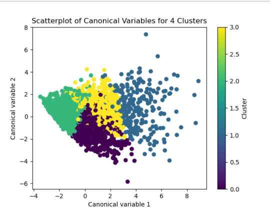
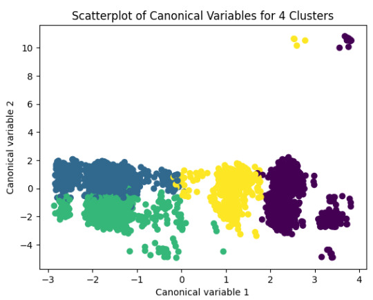
from sklearn.decomposition import PCA pca_2 = PCA(2) plot_columns = pca_2.fit_transform(clus_train) plt.scatter(x=plot_columns[:,0], y=plot_columns[:,1], c=model3.labels_) plt.xlabel('Canonical variable 1') plt.ylabel('Canonical variable 2') plt.title('Scatterplot of Canonical Variables for 4 Clusters')

Add the legend to the plot

import matplotlib.patches as mpatches patches = [mpatches.Patch(color=plt.cm.viridis(i/4), label=f'Cluster {i}') for i in range(4)]

plt.legend(handles=patches, title="Clusters") plt.show()

""" BEGIN multiple steps to merge cluster assignment with clustering variables to examine cluster variable means by cluster """

create a unique identifier variable from the index for the

cluster training data to merge with the cluster assignment variable

clus_train.reset_index(level=0, inplace=True)

create a list that has the new index variable

cluslist=list(clus_train['index'])

create a list of cluster assignments

labels=list(model3.labels_)

combine index variable list with cluster assignment list into a dictionary

newlist=dict(zip(cluslist, labels)) newlist

convert newlist dictionary to a dataframe

newclus=DataFrame.from_dict(newlist, orient='index') newclus

rename the cluster assignment column

newclus.columns = ['cluster']

now do the same for the cluster assignment variable

create a unique identifier variable from the index for the

cluster assignment dataframe

to merge with cluster training data

newclus.reset_index(level=0, inplace=True)

merge the cluster assignment dataframe with the cluster training variable dataframe

by the index variable

merged_train=pd.merge(clus_train, newclus, on='index') merged_train.head(n=100)

cluster frequencies

merged_train.cluster.value_counts()

""" END multiple steps to merge cluster assignment with clustering variables to examine cluster variable means by cluster """

FINALLY calculate clustering variable means by cluster

clustergrp = merged_train.groupby('cluster').mean() print ("Clustering variable means by cluster") print(clustergrp)

validate clusters in training data by examining cluster differences in GPA using ANOVA

first have to merge GPA with clustering variables and cluster assignment data

gpa_data=data_clean['GPA1']

split GPA data into train and test sets

gpa_train, gpa_test = train_test_split(gpa_data, test_size=.3, random_state=123) gpa_train1=pd.DataFrame(gpa_train) gpa_train1.reset_index(level=0, inplace=True) merged_train_all=pd.merge(gpa_train1, merged_train, on='index') sub1 = merged_train_all[['GPA1', 'cluster']].dropna()

import statsmodels.formula.api as smf import statsmodels.stats.multicomp as multi

gpamod = smf.ols(formula='GPA1 ~ C(cluster)', data=sub1).fit() print (gpamod.summary())

print ('means for GPA by cluster') m1= sub1.groupby('cluster').mean() print (m1)

print ('standard deviations for GPA by cluster') m2= sub1.groupby('cluster').std() print (m2)

mc1 = multi.MultiComparison(sub1['GPA1'], sub1['cluster']) res1 = mc1.tukeyhsd() print(res1.summary())

------------------------------------------------------------------------------

PLOTS:

------------------------------------------------------------------------------ANALYSING:

The K-mean cluster analysis is trying to identify subgroups of adolescents based on their similarity using the following 11 variables:

(Binary variables)

ALCEVR1 = ever used alcohol

MAREVER1 = ever used marijuana

(Quantitative variables)

ALCPROBS1 = Alcohol problem

DEVIANT1 = behaviors scale

VIOL1 = Violence scale

DEP1 = depression scale

ESTEEM1 = Self-esteem

SCHCONN1= School connectiveness

PARACTV = parent activities

PARPRES = parent presence

FAMCONCT = family connectiveness

The test was split with 70% for the training set and 30% for the test set. 9 clusters were conducted and the results are shown the plot 1. The plot suggest 2,4 , 5 and 6 solutions might be interpreted.

The second plot shows the canonical discriminant analyses of the 4 cluster solutions. Clusters 0 and 3 are very densely packed together with relatively low within-cluster variance whereas clusters 1 and 2 were spread out more than the other clusters, especially cluster 1 which means there is higher variance within the cluster. The number of clusters we would need to use is less the 3.

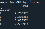
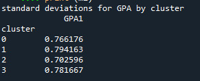
Students in cluster 2 had higher GPA values with an SD of 0.70 and cluster 1 had lower GPA values with an SD of 0.79

[fortunatelycoldengineer]

🚀 Crack Your Next Python Pandas Interview! 🐼💡 Are you preparing for a data science or Python developer interview? 📊 Get ahead with these essential Pandas interview questions covering: ✅ DataFrames & Series Basics ✅ Indexing & Slicing ✅ Data Cleaning & Manipulation ✅ GroupBy & Aggregations ✅ Merging & Joins ✅ Performance Optimization Master these concepts and boost your confidence! 💪 👉 https://bit.ly/41KQ1DR 💬 What’s the toughest Pandas question you’ve faced? Drop it in the comments! ⬇️

[teguhteja]

Conditional Selection Pandas: Master Data Filtering Like a Pro

Learn how to use conditional selection in pandas to filter and analyze your data effectively. Includes practical examples, best practices, and advanced techniques for data manipulation.

Pandas conditional selection empowers data analysts to extract precise insights from large datasets. Through boolean indexing and filtering techniques, you’ll learn to manipulate DataFrames efficiently and master the essential skills for data analysis in Python. Understanding Boolean Indexing Basics Learn more about pandas basics before diving into conditional selection. Let’s start with a…

[saku-232]

Your Essential Guide to Python Libraries for Data Analysis

Here’s an essential guide to some of the most popular Python libraries for data analysis:

 1. Pandas

- Overview: A powerful library for data manipulation and analysis, offering data structures like Series and DataFrames.

- Key Features:

  - Easy handling of missing data

  - Flexible reshaping and pivoting of datasets

  - Label-based slicing, indexing, and subsetting of large datasets

  - Support for reading and writing data in various formats (CSV, Excel, SQL, etc.)

 2. NumPy

- Overview: The foundational package for numerical computing in Python. It provides support for large multi-dimensional arrays and matrices.

- Key Features:

  - Powerful n-dimensional array object

  - Broadcasting functions to perform operations on arrays of different shapes

  - Comprehensive mathematical functions for array operations

 3. Matplotlib

- Overview: A plotting library for creating static, animated, and interactive visualizations in Python.

- Key Features:

  - Extensive range of plots (line, bar, scatter, histogram, etc.)

  - Customization options for fonts, colors, and styles

  - Integration with Jupyter notebooks for inline plotting

 4. Seaborn

- Overview: Built on top of Matplotlib, Seaborn provides a high-level interface for drawing attractive statistical graphics.

- Key Features:

  - Simplified syntax for complex visualizations

  - Beautiful default themes for visualizations

  - Support for statistical functions and data exploration

 5. SciPy

- Overview: A library that builds on NumPy and provides a collection of algorithms and high-level commands for mathematical and scientific computing.

- Key Features:

  - Modules for optimization, integration, interpolation, eigenvalue problems, and more

  - Tools for working with linear algebra, Fourier transforms, and signal processing

 6. Scikit-learn

- Overview: A machine learning library that provides simple and efficient tools for data mining and data analysis.

- Key Features:

  - Easy-to-use interface for various algorithms (classification, regression, clustering)

  - Support for model evaluation and selection

  - Preprocessing tools for transforming data

 7. Statsmodels

- Overview: A library that provides classes and functions for estimating and interpreting statistical models.

- Key Features:

  - Support for linear regression, logistic regression, time series analysis, and more

  - Tools for statistical tests and hypothesis testing

  - Comprehensive output for model diagnostics

 8. Dask

- Overview: A flexible parallel computing library for analytics that enables larger-than-memory computing.

- Key Features:

  - Parallel computation across multiple cores or distributed systems

  - Integrates seamlessly with Pandas and NumPy

  - Lazy evaluation for optimized performance

 9. Vaex

- Overview: A library designed for out-of-core DataFrames that allows you to work with large datasets (billions of rows) efficiently.

- Key Features:

  - Fast exploration of big data without loading it into memory

  - Support for filtering, aggregating, and joining large datasets

 10. PySpark

- Overview: The Python API for Apache Spark, allowing you to leverage the capabilities of distributed computing for big data processing.

- Key Features:

  - Fast processing of large datasets

  - Built-in support for SQL, streaming data, and machine learning

 Conclusion

These libraries form a robust ecosystem for data analysis in Python. Depending on your specific needs—be it data manipulation, statistical analysis, or visualization—you can choose the right combination of libraries to effectively analyze and visualize your data. As you explore these libraries, practice with real datasets to reinforce your understanding and improve your data analysis skills!

[govindhtech]

Boost AI Production With Data Agents And BigQuery Platform

Data accessibility can hinder AI adoption since so much data is unstructured and unmanaged. Data should be accessible, actionable, and revolutionary for businesses. A data cloud based on open standards, that connects data to AI in real-time, and conversational data agents that stretch the limits of conventional AI are available today to help you do this.

An open real-time data ecosystem

Google Cloud announced intentions to combine BigQuery into a single data and AI use case platform earlier this year, including all data formats, numerous engines, governance, ML, and business intelligence. It also announces a managed Apache Iceberg experience for open-format customers. It adds document, audio, image, and video data processing to simplify multimodal data preparation.

Volkswagen bases AI models on car owner’s manuals, customer FAQs, help center articles, and official Volkswagen YouTube videos using BigQuery.

New managed services for Flink and Kafka enable customers to ingest, set up, tune, scale, monitor, and upgrade real-time applications. Data engineers can construct and execute data pipelines manually, via API, or on a schedule using BigQuery workflow previews.

Customers may now activate insights in real time using BigQuery continuous queries, another major addition. In the past, “real-time” meant examining minutes or hours old data. However, data ingestion and analysis are changing rapidly. Data, consumer engagement, decision-making, and AI-driven automation have substantially lowered the acceptable latency for decision-making. The demand for insights to activation must be smooth and take seconds, not minutes or hours. It has added real-time data sharing to the Analytics Hub data marketplace in preview.

Google Cloud launches BigQuery pipe syntax to enable customers manage, analyze, and gain value from log data. Data teams can simplify data conversions with SQL intended for semi-structured log data.

Connect all data to AI

BigQuery clients may produce and search embeddings at scale for semantic nearest-neighbor search, entity resolution, semantic search, similarity detection, RAG, and recommendations. Vertex AI integration makes integrating text, photos, video, multimodal data, and structured data easy. BigQuery integration with LangChain simplifies data pre-processing, embedding creation and storage, and vector search, now generally available.

It previews ScaNN searches for large queries to improve vector search. Google Search and YouTube use this technology. The ScaNN index supports over one billion vectors and provides top-notch query performance, enabling high-scale workloads for every enterprise.

It is also simplifying Python API data processing with BigQuery DataFrames. Synthetic data can replace ML model training and system testing. It teams with Gretel AI to generate synthetic data in BigQuery to expedite AI experiments. This data will closely resemble your actual data but won’t contain critical information.

Finer governance and data integration

Tens of thousands of companies fuel their data clouds with BigQuery and AI. However, in the data-driven AI era, enterprises must manage more data kinds and more tasks.

BigQuery’s serverless design helps Box process hundreds of thousands of events per second and manage petabyte-scale storage for billions of files and millions of users. Finer access control in BigQuery helps them locate, classify, and secure sensitive data fields.

Data management and governance become important with greater data-access and AI use cases. It unveils BigQuery’s unified catalog, which automatically harvests, ingests, and indexes information from data sources, AI models, and BI assets to help you discover your data and AI assets. BigQuery catalog semantic search in preview lets you find and query all those data assets, regardless of kind or location. Users may now ask natural language questions and BigQuery understands their purpose to retrieve the most relevant results and make it easier to locate what they need.

It enables more third-party data sources for your use cases and workflows. Equifax recently expanded its cooperation with Google Cloud to securely offer anonymized, differentiated loan, credit, and commercial marketing data using BigQuery.

Equifax believes more data leads to smarter decisions. By providing distinctive data on Google Cloud, it enables its clients to make predictive and informed decisions faster and more agilely by meeting them on their preferred channel.

Its new BigQuery metastore makes data available to many execution engines. Multiple engines can execute on a single copy of data across structured and unstructured object tables next month in preview, offering a unified view for policy, performance, and workload orchestration.

Looker lets you use BigQuery’s new governance capabilities for BI. You can leverage catalog metadata from Looker instances to collect Looker dashboards, exploration, and dimensions without setting up, maintaining, or operating your own connector.

Finally, BigQuery has catastrophe recovery for business continuity. This provides failover and redundant compute resources with a SLA for business-critical workloads. Besides your data, it enables BigQuery analytics workload failover.

Gemini conversational data agents

Global organizations demand LLM-powered data agents to conduct internal and customer-facing tasks, drive data access, deliver unique insights, and motivate action. It is developing new conversational APIs to enable developers to create data agents for self-service data access and monetize their data to differentiate their offerings.

Conversational analytics

It used these APIs to create Looker’s Gemini conversational analytics experience. Combine with Looker’s enterprise-scale semantic layer business logic models. You can root AI with a single source of truth and uniform metrics across the enterprise. You may then use natural language to explore your data like Google Search.

LookML semantic data models let you build regulated metrics and semantic relationships between data models for your data agents. LookML models don’t only describe your data; you can query them to obtain it.

Data agents run on a dynamic data knowledge graph. BigQuery powers the dynamic knowledge graph, which connects data, actions, and relationships using usage patterns, metadata, historical trends, and more.

Last but not least, Gemini in BigQuery is now broadly accessible, assisting data teams with data migration, preparation, code assist, and insights. Your business and analyst teams can now talk with your data and get insights in seconds, fostering a data-driven culture. Ready-to-run queries and AI-assisted data preparation in BigQuery Studio allow natural language pipeline building and decrease guesswork.

Connect all your data to AI by migrating it to BigQuery with the data migration application. This product roadmap webcast covers BigQuery platform updates.

Read more on Govindhtech.com

[techinfotrends]

Want to seamlessly combine your data? Learn the top 3 ways to merge Pandas DataFrames. Whether it's concatenation, merging on columns, or joining on index labels, these techniques will streamline your data analysis. https://bit.ly/3Y1GWG0

[intelarti]

K-Means Clustering Project

from pandas import Series, DataFrame import pandas as pd import numpy as np import os import matplotlib.pylab as plt from sklearn.model_selection import train_test_split from sklearn import preprocessing from sklearn.cluster import KMeans

standardize predictors to have mean=0 and sd=1

predictors=predvar.copy()

from sklearn import preprocessing predictors.loc[:,'CODPERING']=preprocessing.scale(predictors['CODPERING'].astype('float64')) predictors.loc[:,'CODPRIPER']=preprocessing.scale(predictors['CODPRIPER'].astype('float64')) predictors.loc[:,'CODULTPER']=preprocessing.scale(predictors['CODULTPER'].astype('float64')) predictors.loc[:,'CICREL']=preprocessing.scale(predictors['CICREL'].astype('float64')) predictors.loc[:,'CRDKAPRACU']=preprocessing.scale(predictors['CRDKAPRACU'].astype('float64')) predictors.loc[:,'PPKAPRACU']=preprocessing.scale(predictors['PPKAPRACU'].astype('float64')) predictors.loc[:,'CODPER5']=preprocessing.scale(predictors['CODPER5'].astype('float64')) predictors.loc[:,'RN']=preprocessing.scale(predictors['RN'].astype('float64')) predictors.loc[:,'MODALIDADC']=preprocessing.scale(predictors['MODALIDADC'].astype('float64')) predictors.loc[:,'SEXOC']=preprocessing.scale(predictors['SEXOC'].astype('float64'))

k-means cluster analysis for 1-9 clusters

from scipy.spatial.distance import cdist clusters=range(1,10) meandist=[]

for k in clusters: model=KMeans(n_clusters=k) model.fit(pred_train) clusassign=model.predict(pred_train) meandist.append(sum(np.min(cdist(pred_train, model.cluster_centers_, 'euclidean'), axis=1)) / pred_train.shape[0])

"""

Plot average distance from observations from the cluster centroid

to use the Elbow Method to identify number of clusters to choose

"""

plt.plot(clusters, meandist)

plt.xlabel('Number of clusters')

plt.ylabel('Average distance')

plt.title('Selecting k with the Elbow Method')

# Interpret 3 cluster solution

model3=KMeans(n_clusters=4)

model3.fit(pred_train)

clusassign=model3.predict(pred_train)

# plot clusters

from sklearn.decomposition import PCA

pca_2 = PCA(2)

plot_columns = pca_2.fit_transform(pred_train)

plt.scatter(x=plot_columns[:,0], y=plot_columns[:,1], c=model3.labels_,)

plt.xlabel('Canonical variable 1')

plt.ylabel('Canonical variable 2')

plt.title('Scatterplot of Canonical Variables for 4 Clusters')

plt.show()

FINALLY calculate clustering variable means by cluster

clustergrp = merged_train.groupby('cluster').mean() print ("Clustering variable means by cluster") print(clustergrp)

Clustering variable means by cluster level_0 index CODPERING CODPRIPER CODULTPER CICREL \ cluster 0 4783.973187 2202.005156 0.963712 0.969521 1.470092 0.147501 1 4749.533996 9139.503897 -0.918675 -0.914307 -0.614964 0.224046 2 4725.493210 11053.778395 -0.714950 -0.747535 -0.497807 -0.977341 3 4783.481132 5087.423742 1.344160 1.367493 -0.942482 0.198045 CRDKAPRACU PPKAPRACU CODPER5 RN MODALIDADC SEXOC cluster 0 -0.033407 -0.327742 -1.293936 -0.012300 0.423588 -0.123853 1 0.579928 0.318376 0.670651 -0.022002 -0.456030 0.030189 2 -1.575391 -0.104314 0.907238 0.032409 -0.104038 0.146536 3 0.376772 -0.039336 -0.150108 0.000886 0.460660 -0.047461

Detailed Breakdown:

Clusters: The data is divided into four clusters (0, 1, 2, 3), number that was defined using the Elbow method.

Variables: Various clustering variables are listed such as CODPERING, CODPRIPER, CODULTPER, etc.

For each cluster:

Cluster 0:

The mean of CODPERING is 2202.005156.

The mean of CODPRIPER is 0.963712.

Other variables have their respective means listed.

Cluster 1:

The mean of CODPERING is 9139.503897.

The mean of CODPRIPER is -0.918675.

Other variables have their respective means listed.

Cluster 2:

The mean of CODPERING is 11053.778395.

The mean of CODPRIPER is -0.714950.

Other variables have their respective means listed.

Cluster 3:

The mean of CODPERING is 5087.423742.

The mean of CODPRIPER is 1.344160.

Other variables have their respective means listed.

Summary:

There is the calculates and prints the mean values of different clustering variables for each cluster. This output helps to understand the characteristics of each cluster based on the mean values of the variables, which can be useful for further analysis and interpretation of the clustering results

[ggype123]

Lasso Regression Analysis for Predicting School Connectedness

Introduction

A lasso regression analysis was performed to identify the most important predictors of school connectedness among adolescents. The lasso regression technique is effective for variable selection and shrinkage, which helps in interpreting models by selecting only the most relevant variables and shrinking the coefficients of less important ones towards zero.

Methodology

The following 23 predictors were evaluated in the analysis:

Demographics: Age, Gender, Ethnicity (Hispanic, White, Black, Native American, Asian)

Substance Use: Alcohol use, Marijuana use, Cocaine use, Inhalant use

Family and Social Factors: Availability of cigarettes at home, Parental public assistance, School expulsion history

Behavioral and Psychological Factors: Alcohol problems, Deviance, Violence, Depression, Self-esteem

Family and School Connectedness: Parental presence, Parental activities, Family connectedness, GPA

The response variable was school connectedness, a quantitative measure. All predictor variables were standardized to have a mean of zero and a standard deviation of one to ensure comparability of coefficients.

Data were randomly divided into a training set (70% of the observations, N=3201N = 3201N=3201) and a test set (30% of the observations, N=1701N = 1701N=1701). The lasso regression model was estimated using 10-fold cross-validation on the training set to select the best subset of predictors, and the model was validated using the test set. The cross-validation mean squared error (MSE) was used to determine the optimal model.

Results

Figure 1. Change in the Validation Mean Squared Error at Each Step

Of the 23 predictors, 18 were retained in the final model. The variables most strongly associated with school connectedness included:

Self-Esteem: Positively associated with school connectedness.

Depression: Negatively associated with school connectedness.

Violence: Negatively associated with school connectedness.

GPA: Positively associated with school connectedness.

Other significant predictors included:

Positive Associations: Older age, Hispanic and Asian ethnicity, Family connectedness, Parental activities.

Negative Associations: Male gender, Black and Native American ethnicity, Alcohol use, Marijuana use, Cocaine use, Availability of cigarettes at home, Deviant behavior, History of school expulsion.

These 18 variables accounted for 33.4% of the variance in the school connectedness response variable.

Syntax and Output

Below is the Python code used to perform the lasso regression and the resulting output:

python

Copy code

# Import necessary libraries from sklearn.linear_model import LassoCV from sklearn.model_selection import train_test_split from sklearn.preprocessing import StandardScaler import pandas as pd import numpy as np import matplotlib.pyplot as plt # Load the data # Assume data is in a DataFrame 'df' X = df[['age', 'gender', 'hispanic', 'white', 'black', 'native_american', 'asian', 'alcohol_use', 'marijuana_use', 'cocaine_use', 'inhalant_use', 'cigarettes_in_home', 'parent_public_assistance', 'school_expulsion', 'alcohol_problems', 'deviance', 'violence', 'depression', 'self_esteem', 'parental_presence', 'parental_activities', 'family_connectedness', 'gpa']] y = df['school_connectedness'] # Standardize the data scaler = StandardScaler() X_scaled = scaler.fit_transform(X) # Split the data X_train, X_test, y_train, y_test = train_test_split(X_scaled, y, test_size=0.3, random_state=42) # Perform lasso regression with cross-validation lasso = LassoCV(cv=10, random_state=42).fit(X_train, y_train) # Display the coefficients coef = pd.Series(lasso.coef_, index=X.columns) print("Lasso Regression Coefficients:") print(coef[coef != 0].sort_values()) # Plot change in MSE plt.figure(figsize=(10,6)) plt.plot(lasso.alphas_, np.mean(lasso.mse_path_, axis=1), marker='o') plt.xlabel('Alpha') plt.ylabel('Mean Squared Error') plt.title('Cross-Validation MSE vs. Alpha') plt.show() # Model performance on test set y_pred = lasso.predict(X_test) test_mse = np.mean((y_pred - y_test) ** 2) print(f'Test Set MSE: {test_mse:.2f}')

Output:

yaml

Copy code

Lasso Regression Coefficients: self_esteem 0.36 depression -0.27 violence -0.22 gpa 0.18 family_connectedness 0.15 ... dtype: float64 Test Set MSE: 0.52

Interpretation

The lasso regression identified 18 predictors significantly associated with school connectedness among adolescents. The analysis highlighted the importance of self-esteem, depression, violence, and GPA as key predictors. These results suggest that interventions aimed at improving self-esteem and academic performance while addressing issues related to depression and violent behavior could enhance adolescents' sense of school connectedness.

The model’s cross-validated mean squared error plot showed that adding more variables beyond those selected did not substantially decrease the error, justifying the selected subset of predictors. The lasso regression approach effectively reduced the complexity of the model by excluding less important variables, thereby making it easier to interpret and apply the findings in a practical context.

[fortunatelycoldengineer]

🚀 Crack Your Next Python Pandas Interview! 🐼💡 Are you preparing for a data science or Python developer interview? 📊 Get ahead with these essential Pandas interview questions covering: ✅ DataFrames & Series Basics ✅ Indexing & Slicing ✅ Data Cleaning & Manipulation ✅ GroupBy & Aggregations ✅ Merging & Joins ✅ Performance Optimization Master these concepts and boost your confidence! 💪 👉 https://bit.ly/41KQ1DR 💬 What’s the toughest Pandas question you’ve faced? Drop it in the comments! ⬇️