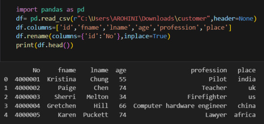
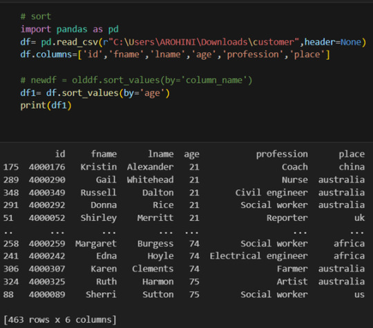
#rename columns in pandas dataframe

[codewithnazam]

DataFrame in Pandas: Guide to Creating Awesome DataFrames

Explore how to create a dataframe in Pandas, including data input methods, customization options, and practical examples.

Data analysis used to be a daunting task, reserved for statisticians and mathematicians. But with the rise of powerful tools like Python and its fantastic library, Pandas, anyone can become a data whiz! Pandas, in particular, shines with its DataFrames, these nifty tables that organize and manipulate data like magic. But where do you start? Fear not, fellow data enthusiast, for this guide will…

[tia003]

How To Use Pandas For Analysis?

Pandas is a powerful Python library used for data manipulation and analysis. It provides two primary data structures: Series (one-dimensional) and DataFrame (two-dimensional), which are essential for handling structured data. To start using Pandas, first import it using import pandas as pd. You can then load data from various sources such as CSV, Excel, or SQL databases using functions like pd.read_csv() or pd.read_excel().

Once your data is loaded into a DataFrame, you can explore it with methods like .head(), .info(), and .describe() to get a quick summary. Cleaning data involves handling missing values (.dropna(), .fillna()), renaming columns, or changing data types. For analysis, you can use filtering (df[df['column'] > value]), grouping (.groupby()), and aggregation functions (.mean(), .sum(), .count()). Visualization libraries like Matplotlib or Seaborn can be used alongside Pandas to plot the data for deeper insights.

Pandas is essential for data analysts, making it easier to understand patterns and trends in datasets. If you're new to this, consider starting with a Python course for beginners to build a solid foundation.

[machinelearningcoursera]

K-mean Analysis

Script:

from pandas import Series, DataFrame import pandas as pd import numpy as np import matplotlib.pylab as plt from sklearn.model_selection import train_test_split from sklearn import preprocessing from sklearn.cluster import KMeans import os """ Data Management """

data = pd.read_csv("tree_addhealth.csv")

upper-case all DataFrame column names

data.columns = map(str.upper, data.columns)

Data Management

data_clean = data.dropna()

subset clustering variables

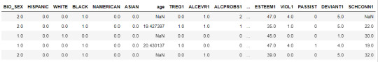
cluster=data_clean[['ALCEVR1','MAREVER1','ALCPROBS1','DEVIANT1','VIOL1', 'DEP1','ESTEEM1','SCHCONN1','PARACTV', 'PARPRES','FAMCONCT']] cluster.describe()

standardize clustering variables to have mean=0 and sd=1

clustervar=cluster.copy() clustervar['ALCEVR1']=preprocessing.scale(clustervar['ALCEVR1'].astype('float64')) clustervar['ALCPROBS1']=preprocessing.scale(clustervar['ALCPROBS1'].astype('float64')) clustervar['MAREVER1']=preprocessing.scale(clustervar['MAREVER1'].astype('float64')) clustervar['DEP1']=preprocessing.scale(clustervar['DEP1'].astype('float64')) clustervar['ESTEEM1']=preprocessing.scale(clustervar['ESTEEM1'].astype('float64')) clustervar['VIOL1']=preprocessing.scale(clustervar['VIOL1'].astype('float64')) clustervar['DEVIANT1']=preprocessing.scale(clustervar['DEVIANT1'].astype('float64')) clustervar['FAMCONCT']=preprocessing.scale(clustervar['FAMCONCT'].astype('float64')) clustervar['SCHCONN1']=preprocessing.scale(clustervar['SCHCONN1'].astype('float64')) clustervar['PARACTV']=preprocessing.scale(clustervar['PARACTV'].astype('float64')) clustervar['PARPRES']=preprocessing.scale(clustervar['PARPRES'].astype('float64'))

split data into train and test sets

clus_train, clus_test = train_test_split(clustervar, test_size=.3, random_state=123)

k-means cluster analysis for 1-9 clusters

from scipy.spatial.distance import cdist clusters=range(1,9) meandist=[]

for k in clusters: model=KMeans(n_clusters=k) model.fit(clus_train) clusassign=model.predict(clus_train) meandist.append(sum(np.min(cdist(clus_train, model.cluster_centers_, 'euclidean'), axis=1)) / clus_train.shape[0])

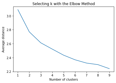
""" Plot average distance from observations from the cluster centroid to use the Elbow Method to identify number of clusters to choose """

plt.plot(clusters, meandist) plt.xlabel('Number of clusters') plt.ylabel('Average distance') plt.title('Selecting k with the Elbow Method')

Interpret 3 cluster solution

model3=KMeans(n_clusters=2) model3.fit(clus_train) clusassign=model3.predict(clus_train)

plot clusters

from sklearn.decomposition import PCA pca_2 = PCA(2) plot_columns = pca_2.fit_transform(clus_train) plt.scatter(x=plot_columns[:,0], y=plot_columns[:,1], c=model3.labels_) plt.xlabel('Canonical variable 1') plt.ylabel('Canonical variable 2') plt.title('Scatterplot of Canonical Variables for 4 Clusters')

Add the legend to the plot

import matplotlib.patches as mpatches patches = [mpatches.Patch(color=plt.cm.viridis(i/4), label=f'Cluster {i}') for i in range(4)]

plt.legend(handles=patches, title="Clusters") plt.show()

""" BEGIN multiple steps to merge cluster assignment with clustering variables to examine cluster variable means by cluster """

create a unique identifier variable from the index for the

cluster training data to merge with the cluster assignment variable

clus_train.reset_index(level=0, inplace=True)

create a list that has the new index variable

cluslist=list(clus_train['index'])

create a list of cluster assignments

labels=list(model3.labels_)

combine index variable list with cluster assignment list into a dictionary

newlist=dict(zip(cluslist, labels)) newlist

convert newlist dictionary to a dataframe

newclus=DataFrame.from_dict(newlist, orient='index') newclus

rename the cluster assignment column

newclus.columns = ['cluster']

now do the same for the cluster assignment variable

create a unique identifier variable from the index for the

cluster assignment dataframe

to merge with cluster training data

newclus.reset_index(level=0, inplace=True)

merge the cluster assignment dataframe with the cluster training variable dataframe

by the index variable

merged_train=pd.merge(clus_train, newclus, on='index') merged_train.head(n=100)

cluster frequencies

merged_train.cluster.value_counts()

""" END multiple steps to merge cluster assignment with clustering variables to examine cluster variable means by cluster """

FINALLY calculate clustering variable means by cluster

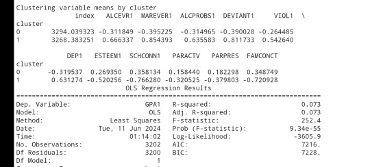
clustergrp = merged_train.groupby('cluster').mean() print ("Clustering variable means by cluster") print(clustergrp)

validate clusters in training data by examining cluster differences in GPA using ANOVA

first have to merge GPA with clustering variables and cluster assignment data

gpa_data=data_clean['GPA1']

split GPA data into train and test sets

gpa_train, gpa_test = train_test_split(gpa_data, test_size=.3, random_state=123) gpa_train1=pd.DataFrame(gpa_train) gpa_train1.reset_index(level=0, inplace=True) merged_train_all=pd.merge(gpa_train1, merged_train, on='index') sub1 = merged_train_all[['GPA1', 'cluster']].dropna()

import statsmodels.formula.api as smf import statsmodels.stats.multicomp as multi

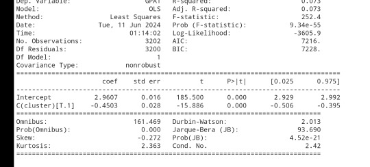
gpamod = smf.ols(formula='GPA1 ~ C(cluster)', data=sub1).fit() print (gpamod.summary())

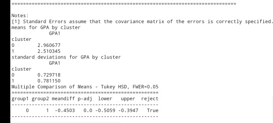
print ('means for GPA by cluster') m1= sub1.groupby('cluster').mean() print (m1)

print ('standard deviations for GPA by cluster') m2= sub1.groupby('cluster').std() print (m2)

mc1 = multi.MultiComparison(sub1['GPA1'], sub1['cluster']) res1 = mc1.tukeyhsd() print(res1.summary())

------------------------------------------------------------------------------

PLOTS:

------------------------------------------------------------------------------ANALYSING:

The K-mean cluster analysis is trying to identify subgroups of adolescents based on their similarity using the following 11 variables:

(Binary variables)

ALCEVR1 = ever used alcohol

MAREVER1 = ever used marijuana

(Quantitative variables)

ALCPROBS1 = Alcohol problem

DEVIANT1 = behaviors scale

VIOL1 = Violence scale

DEP1 = depression scale

ESTEEM1 = Self-esteem

SCHCONN1= School connectiveness

PARACTV = parent activities

PARPRES = parent presence

FAMCONCT = family connectiveness

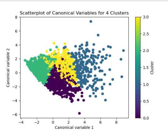
The test was split with 70% for the training set and 30% for the test set. 9 clusters were conducted and the results are shown the plot 1. The plot suggest 2,4 , 5 and 6 solutions might be interpreted.

The second plot shows the canonical discriminant analyses of the 4 cluster solutions. Clusters 0 and 3 are very densely packed together with relatively low within-cluster variance whereas clusters 1 and 2 were spread out more than the other clusters, especially cluster 1 which means there is higher variance within the cluster. The number of clusters we would need to use is less the 3.

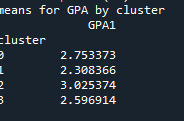
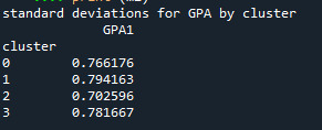
Students in cluster 2 had higher GPA values with an SD of 0.70 and cluster 1 had lower GPA values with an SD of 0.79

[tutorialwithexample]

Unlock the Power of Pandas: Easy-to-Follow Python Tutorial for Newbies

Python Pandas is a powerful tool for working with data, making it a must-learn library for anyone starting in data analysis. With Pandas, you can effortlessly clean, organize, and analyze data to extract meaningful insights. This tutorial is perfect for beginners looking to get started with Pandas.

Pandas is a Python library designed specifically for data manipulation and analysis. It offers two main data structures: Series and DataFrame. A Series is like a single column of data, while a DataFrame is a table-like structure that holds rows and columns, similar to a spreadsheet.

Why use Pandas? First, it simplifies handling large datasets by providing easy-to-use functions for filtering, sorting, and grouping data. Second, it works seamlessly with other popular Python libraries, such as NumPy and Matplotlib, making it a versatile tool for data projects.

Getting started with Pandas is simple. After installing the library, you can load datasets from various sources like CSV files, Excel sheets, or even databases. Once loaded, Pandas lets you perform tasks like renaming columns, replacing missing values, or summarizing data in just a few lines of code.

If you're looking to dive deeper into how Pandas can make your data analysis journey smoother, explore this beginner-friendly guide: Python Pandas Tutorial. Start your journey today, and unlock the potential of data analysis with Python Pandas!

Whether you're a student or a professional, mastering Pandas will open doors to numerous opportunities in the world of data science.

[mengchunhsieh]

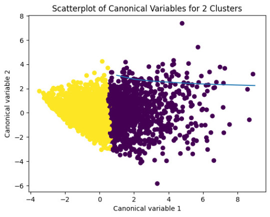
K-means clusthering

#importamos las librerías necesarias

from pandas import Series,DataFrame

import pandas as pd

import numpy as np

import matplotlib.pylab as plt

from sklearn.model_selection

import train_test_splitfrom sklearn

import preprocessing

from sklearn.cluster import KMeans

"""Data Management"""

data =pd.read_csv("/content/drive/MyDrive/tree_addhealth.csv" )

#upper-case all DataFrame column names

data.columns = map(str.upper, data.columns)

# Data Managementdata_clean = data.dropna()

# subset clustering variablescluster=data_clean[['ALCEVR1','MAREVER1','ALCPROBS1','DEVIANT1','VIOL1','DEP1','ESTEEM1','SCHCONN1','PARACTV', 'PARPRES','FAMCONCT']]

cluster.describe()

# standardize clustering variables to have mean=0 and sd=1

clustervar=cluster.copy()

clustervar['ALCEVR1']=preprocessing.scale(clustervar['ALCEVR1'].astype('float64'))

clustervar['ALCPROBS1']=preprocessing.scale(clustervar['ALCPROBS1'].astype('float64'))

clustervar['MAREVER1']=preprocessing.scale(clustervar['MAREVER1'].astype('float64'))

clustervar['DEP1']=preprocessing.scale(clustervar['DEP1'].astype('float64'))

clustervar['ESTEEM1']=preprocessing.scale(clustervar['ESTEEM1'].astype('float64'))

clustervar['VIOL1']=preprocessing.scale(clustervar['VIOL1'].astype('float64'))

clustervar['DEVIANT1']=preprocessing.scale(clustervar['DEVIANT1'].astype('float64'))

clustervar['FAMCONCT']=preprocessing.scale(clustervar['FAMCONCT'].astype('float64'))

clustervar['SCHCONN1']=preprocessing.scale(clustervar['SCHCONN1'].astype('float64'))

clustervar['PARACTV']=preprocessing.scale(clustervar['PARACTV'].astype('float64'))

clustervar['PARPRES']=preprocessing.scale(clustervar['PARPRES'].astype('float64'))

# split data into train and test sets

clus_train, clus_test = train_test_split(clustervar, test_size=.3, random_state=123)

# k-means cluster analysis for 1-9 clusters

from scipy.spatial.distance import cdist

clusters=range(1,10)

meandist=[]

for k in clusters: model=KMeans(n_clusters=k) model.fit(clus_train) clusassign=model.predict(clus_train) meandist.append(sum(np.min(cdist(clus_train, model.cluster_centers_, 'euclidean'), axis=1))

/ clus_train.shape[0])

"""Plot average distance from observations from the cluster centroidto use the Elbow Method to identify number of clusters to choose"""

plt.plot(clusters,meandist)

plt.xlabel('Number of clusters')

plt.ylabel('Average distance')

plt.title('Selecting k with the Elbow Method')

# Interpret 2 cluster solution

model2=KMeans(n_clusters=2)model2.fit(clus_train)

clusassign=model2.predict(clus_train)

# plot clusters

from sklearn.decomposition import PCA

pca_2 = PCA(2)

plot_columns = pca_2.fit_transform(clus_train)

plt.scatter(x=plot_columns[:,0],y=plot_columns[:,1],c=model2.labels_,)

plt.xlabel('Canonical variable 1')

plt.ylabel('Canonical variable 2')

plt.title('Scatterplot of Canonical Variables for 2 Clusters')

plt.show()

"""BEGIN multiple steps to merge cluster assignment with clustering variables to examinecluster variable means by cluster"""

# create a unique identifier variable from the index for the

# cluster training data to merge with the cluster assignment variable

clus_train.reset_index(level=0, inplace=True)

# create a list that has the new index variable

cluslist=list(clus_train['index'])

# create a list of cluster assignments

labels=list(model2.labels_)

# combine index variable list with cluster assignment list into a dictionary

newlist=dict(zip(cluslist, labels))newlist

# convert newlist dictionary to a dataframenew

clus=DataFrame.from_dict(newlist, orient='index')newclus

# rename the cluster assignment columnnew

clus.columns = ['cluster']

# now do the same for the cluster assignment variable

# create a unique identifier variable from the index for the

# cluster assignment dataframe

# to merge with cluster training datanew

clus.reset_index(level=0, inplace=True)

# merge the cluster assignment dataframe with the cluster training variable dataframe

# by the index variablemerged_train=pd.merge(clus_train, newclus, on='index')

merged_train.head(n=100)

# cluster frequenciesmerged_train.cluster.value_counts()

"""END multiple steps to merge cluster assignment with clustering variables to examinecluster variable means by cluster"""

# FINALLY calculate clustering variable means by

clusterclustergrp = merged_train.groupby('cluster').mean()print ("Clustering variable means by cluster")

print(clustergrp)

# validate clusters in training data by examining cluster differences in GPA using ANOVA

# first have to merge GPA with clustering variables and cluster assignment data

gpa_data=data_clean['GPA1']

# split GPA data into train and test sets

gpa_train, gpa_test = train_test_split(gpa_data, test_size=.3, random_state=123)

gpa_train1=pd.DataFrame(gpa_train)

gpa_train1.reset_index(level=0, inplace=True)

merged_train_all=pd.merge(gpa_train1, merged_train, on='index')

sub1 = merged_train_all[['GPA1', 'cluster']].dropna()

import statsmodels.formula.api as smf

import statsmodels.stats.multicomp as multi

gpamod = smf.ols(formula='GPA1 ~ C(cluster)', data=sub1).fit()

print (gpamod.summary())

print ('means for GPA by cluster')

m1= sub1.groupby('cluster').mean()

print (m1)

print ('standard deviations for GPA by cluster')

m2= sub1.groupby('cluster').std()print (m2)

mc1 = multi.MultiComparison(sub1['GPA1'], sub1['cluster'])

res1 = mc1.tukeyhsd()

print(res1.summary())

爆發

0 則迴響

[rogerscode]

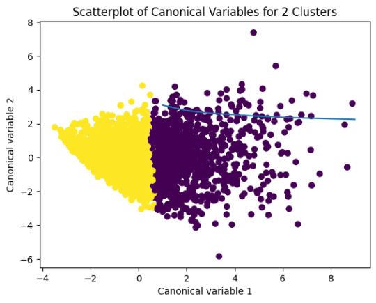
K-means clusthering

#importamos las librerías necesarias

from pandas import Series,DataFrame

import pandas as pd

import numpy as np

import matplotlib.pylab as plt

from sklearn.model_selection

import train_test_splitfrom sklearn

import preprocessing

from sklearn.cluster import KMeans

"""Data Management"""

data =pd.read_csv("/content/drive/MyDrive/tree_addhealth.csv" )

#upper-case all DataFrame column names

data.columns = map(str.upper, data.columns)

# Data Managementdata_clean = data.dropna()

# subset clustering variablescluster=data_clean[['ALCEVR1','MAREVER1','ALCPROBS1','DEVIANT1','VIOL1','DEP1','ESTEEM1','SCHCONN1','PARACTV', 'PARPRES','FAMCONCT']]

cluster.describe()

# standardize clustering variables to have mean=0 and sd=1

clustervar=cluster.copy()

clustervar['ALCEVR1']=preprocessing.scale(clustervar['ALCEVR1'].astype('float64'))

clustervar['ALCPROBS1']=preprocessing.scale(clustervar['ALCPROBS1'].astype('float64'))

clustervar['MAREVER1']=preprocessing.scale(clustervar['MAREVER1'].astype('float64'))

clustervar['DEP1']=preprocessing.scale(clustervar['DEP1'].astype('float64'))

clustervar['ESTEEM1']=preprocessing.scale(clustervar['ESTEEM1'].astype('float64'))

clustervar['VIOL1']=preprocessing.scale(clustervar['VIOL1'].astype('float64'))

clustervar['DEVIANT1']=preprocessing.scale(clustervar['DEVIANT1'].astype('float64'))

clustervar['FAMCONCT']=preprocessing.scale(clustervar['FAMCONCT'].astype('float64'))

clustervar['SCHCONN1']=preprocessing.scale(clustervar['SCHCONN1'].astype('float64'))

clustervar['PARACTV']=preprocessing.scale(clustervar['PARACTV'].astype('float64'))

clustervar['PARPRES']=preprocessing.scale(clustervar['PARPRES'].astype('float64'))

# split data into train and test sets

clus_train, clus_test = train_test_split(clustervar, test_size=.3, random_state=123)

# k-means cluster analysis for 1-9 clusters

from scipy.spatial.distance import cdist

clusters=range(1,10)

meandist=[]

for k in clusters: model=KMeans(n_clusters=k) model.fit(clus_train) clusassign=model.predict(clus_train) meandist.append(sum(np.min(cdist(clus_train, model.cluster_centers_, 'euclidean'), axis=1))

/ clus_train.shape[0])

"""Plot average distance from observations from the cluster centroidto use the Elbow Method to identify number of clusters to choose"""

plt.plot(clusters,meandist)

plt.xlabel('Number of clusters')

plt.ylabel('Average distance')

plt.title('Selecting k with the Elbow Method')

# Interpret 2 cluster solution

model2=KMeans(n_clusters=2)model2.fit(clus_train)

clusassign=model2.predict(clus_train)

# plot clusters

from sklearn.decomposition import PCA

pca_2 = PCA(2)

plot_columns = pca_2.fit_transform(clus_train)

plt.scatter(x=plot_columns[:,0],y=plot_columns[:,1],c=model2.labels_,)

plt.xlabel('Canonical variable 1')

plt.ylabel('Canonical variable 2')

plt.title('Scatterplot of Canonical Variables for 2 Clusters')

plt.show()

"""BEGIN multiple steps to merge cluster assignment with clustering variables to examinecluster variable means by cluster"""

# create a unique identifier variable from the index for the

# cluster training data to merge with the cluster assignment variable

clus_train.reset_index(level=0, inplace=True)

# create a list that has the new index variable

cluslist=list(clus_train['index'])

# create a list of cluster assignments

labels=list(model2.labels_)

# combine index variable list with cluster assignment list into a dictionary

newlist=dict(zip(cluslist, labels))newlist

# convert newlist dictionary to a dataframenew

clus=DataFrame.from_dict(newlist, orient='index')newclus

# rename the cluster assignment columnnew

clus.columns = ['cluster']

# now do the same for the cluster assignment variable

# create a unique identifier variable from the index for the

# cluster assignment dataframe

# to merge with cluster training datanew

clus.reset_index(level=0, inplace=True)

# merge the cluster assignment dataframe with the cluster training variable dataframe

# by the index variablemerged_train=pd.merge(clus_train, newclus, on='index')

merged_train.head(n=100)

# cluster frequenciesmerged_train.cluster.value_counts()

"""END multiple steps to merge cluster assignment with clustering variables to examinecluster variable means by cluster"""

# FINALLY calculate clustering variable means by

clusterclustergrp = merged_train.groupby('cluster').mean()print ("Clustering variable means by cluster")

print(clustergrp)

# validate clusters in training data by examining cluster differences in GPA using ANOVA

# first have to merge GPA with clustering variables and cluster assignment data

gpa_data=data_clean['GPA1']

# split GPA data into train and test sets

gpa_train, gpa_test = train_test_split(gpa_data, test_size=.3, random_state=123)

gpa_train1=pd.DataFrame(gpa_train)

gpa_train1.reset_index(level=0, inplace=True)

merged_train_all=pd.merge(gpa_train1, merged_train, on='index')

sub1 = merged_train_all[['GPA1', 'cluster']].dropna()

import statsmodels.formula.api as smf

import statsmodels.stats.multicomp as multi

gpamod = smf.ols(formula='GPA1 ~ C(cluster)', data=sub1).fit()

print (gpamod.summary())

print ('means for GPA by cluster')

m1= sub1.groupby('cluster').mean()

print (m1)

print ('standard deviations for GPA by cluster')

m2= sub1.groupby('cluster').std()print (m2)

mc1 = multi.MultiComparison(sub1['GPA1'], sub1['cluster'])

res1 = mc1.tukeyhsd()

print(res1.summary())

[asquaretechnologies]

Beginner’s Guide: Data Analysis with Pandas

Data analysis is the process of sorting through all the data, looking for patterns, connections, and interesting things. It helps us make sense of information and use it to make decisions or find solutions to problems. When it comes to data analysis and manipulation in Python, the Pandas library reigns supreme. Pandas provide powerful tools for working with structured data, making it an indispensable asset for both beginners and experienced data scientists.

What is Pandas?

Pandas is an open-source Python library for data manipulation and analysis. It is built on top of NumPy, another popular numerical computing library, and offers additional features specifically tailored for data manipulation and analysis. There are two primary data structures in Pandas:

• Series: A one-dimensional array capable of holding any type of data.

• DataFrame: A two-dimensional labeled data structure similar to a table in relational databases.

It allows us to efficiently process and analyze data, whether it comes from any file types like CSV files, Excel spreadsheets, SQL databases, etc.

How to install Pandas?

We can install Pandas using the pip command. We can run the following codes in the terminal.

After installing, we can import it using:

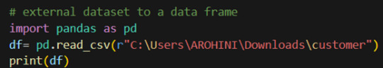
How to load an external dataset using Pandas?

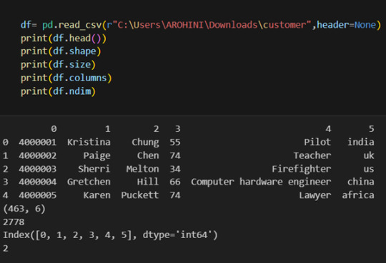
Pandas provide various functions for loading data into a data frame. One of the most commonly used functions is pd.read_csv() for reading CSV files. For example:

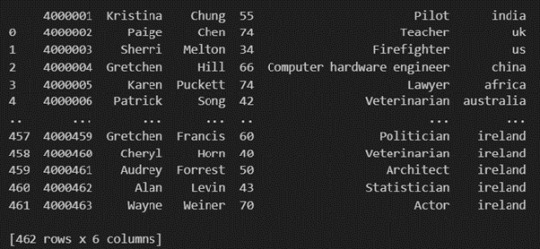
The output of the above code is:

Once your data is loaded into a data frame, you can start exploring it. Pandas offers numerous methods and attributes for getting insights into your data. Here are a few examples:

df.head(): View the first few rows of the DataFrame.

df.tail(): View the last few rows of the DataFrame.

http://df.info(): Get a concise summary of the DataFrame, including data types and missing values.

df.describe(): Generate descriptive statistics for numerical columns.

df.shape: Get the dimensions of the DataFrame (rows, columns).

df.columns: Access the column labels of the DataFrame.

df.dtypes: Get the data types of each column.

In data analysis, it is essential to do data cleaning. Pandas provide powerful tools for handling missing data, removing duplicates, and transforming data. Some common data-cleaning tasks include:

Handling missing values using methods like df.dropna() or df.fillna().

Removing duplicate rows with df.drop_duplicates().

Data type conversion using df.astype().

Renaming columns with df.rename().

Pandas excels in data manipulation tasks such as selecting subsets of data, filtering rows, and creating new columns. Here are a few examples:

Selecting columns: df[‘column_name’] or df[[‘column1’, ‘column2’]].

Filtering rows based on conditions: df[df[‘column’] > value].

Sorting data: df.sort_values(by=’column’).

Grouping data: df.groupby(‘column’).mean().

With data cleaned and prepared, you can use Pandas to perform various analyses. Whether you’re computing statistics, performing exploratory data analysis, or building predictive models, Pandas provides the tools you need. Additionally, Pandas integrates seamlessly with other libraries such as Matplotlib and Seaborn for data visualization

[deba1407]

KMeans Clustering Assignment

Import the modules

from pandas import Series, DataFrame import pandas as pd import numpy as np import matplotlib.pylab as plt from sklearn.model_selection import train_test_split from sklearn import preprocessing from sklearn.cluster import KMeans

Load the dataset

data = pd.read_csv("C:\Users\guy3404\OneDrive - MDLZ\Documents\Cross Functional Learning\AI COP\Coursera\machine_learning_data_analysis\Datasets\tree_addhealth.csv")

data.head()

upper-case all DataFrame column names

data.columns = map(str.upper, data.columns)

Data Management

data_clean = data.dropna() data_clean.head()

subset clustering variables

cluster=data_clean[['ALCEVR1','MAREVER1','ALCPROBS1','DEVIANT1','VIOL1', 'DEP1','ESTEEM1','SCHCONN1','PARACTV', 'PARPRES','FAMCONCT']] cluster.describe()

standardize clustering variables to have mean=0 and sd=1

clustervar=cluster.copy() clustervar['ALCEVR1']=preprocessing.scale(clustervar['ALCEVR1'].astype('float64')) clustervar['ALCPROBS1']=preprocessing.scale(clustervar['ALCPROBS1'].astype('float64')) clustervar['MAREVER1']=preprocessing.scale(clustervar['MAREVER1'].astype('float64')) clustervar['DEP1']=preprocessing.scale(clustervar['DEP1'].astype('float64')) clustervar['ESTEEM1']=preprocessing.scale(clustervar['ESTEEM1'].astype('float64')) clustervar['VIOL1']=preprocessing.scale(clustervar['VIOL1'].astype('float64')) clustervar['DEVIANT1']=preprocessing.scale(clustervar['DEVIANT1'].astype('float64')) clustervar['FAMCONCT']=preprocessing.scale(clustervar['FAMCONCT'].astype('float64')) clustervar['SCHCONN1']=preprocessing.scale(clustervar['SCHCONN1'].astype('float64')) clustervar['PARACTV']=preprocessing.scale(clustervar['PARACTV'].astype('float64')) clustervar['PARPRES']=preprocessing.scale(clustervar['PARPRES'].astype('float64'))

split data into train and test sets

clus_train, clus_test = train_test_split(clustervar, test_size=.3, random_state=123)

k-means cluster analysis for 1-9 clusters

from scipy.spatial.distance import cdist clusters=range(1,10) meandist=[]

for k in clusters: model=KMeans(n_clusters=k) model.fit(clus_train) clusassign=model.predict(clus_train) meandist.append(sum(np.min(cdist(clus_train, model.cluster_centers_, 'euclidean'), axis=1)) / clus_train.shape[0])

""" Plot average distance from observations from the cluster centroid to use the Elbow Method to identify number of clusters to choose """ plt.plot(clusters, meandist) plt.xlabel('Number of clusters') plt.ylabel('Average distance') plt.title('Selecting k with the Elbow Method')

Interpret 3 cluster solution

model3=KMeans(n_clusters=3) model3.fit(clus_train) clusassign=model3.predict(clus_train)

plot clusters

from sklearn.decomposition import PCA pca_2 = PCA(2) plot_columns = pca_2.fit_transform(clus_train) plt.scatter(x=plot_columns[:,0], y=plot_columns[:,1], c=model3.labels_,) plt.xlabel('Canonical variable 1') plt.ylabel('Canonical variable 2') plt.title('Scatterplot of Canonical Variables for 3 Clusters') plt.show()

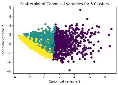
The datapoints of the 2 clusters in the left are less spread out but have more overlaps. The cluster to the right is more distinct but has more spread in the data points

""" BEGIN multiple steps to merge cluster assignment with clustering variables to examine cluster variable means by cluster """

create a unique identifier variable from the index for the

cluster training data to merge with the cluster assignment variable

clus_train.reset_index(level=0, inplace=True)

create a list that has the new index variable

cluslist=list(clus_train['index'])

create a list of cluster assignments

labels=list(model3.labels_)

combine index variable list with cluster assignment list into a dictionary

newlist=dict(zip(cluslist, labels)) newlist

convert newlist dictionary to a dataframe

newclus=DataFrame.from_dict(newlist, orient='index') newclus

rename the cluster assignment column

newclus.columns = ['cluster']

now do the same for the cluster assignment variable

create a unique identifier variable from the index for the

cluster assignment dataframe

to merge with cluster training data

newclus.reset_index(level=0, inplace=True)

merge the cluster assignment dataframe with the cluster training variable dataframe

by the index variable

merged_train=pd.merge(clus_train, newclus, on='index') merged_train.head(n=100)

cluster frequencies

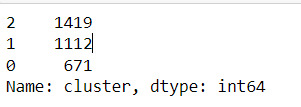
merged_train.cluster.value_counts()

""" END multiple steps to merge cluster assignment with clustering variables to examine cluster variable means by cluster """

FINALLY calculate clustering variable means by cluster

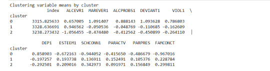
clustergrp = merged_train.groupby('cluster').mean() print ("Clustering variable means by cluster") print(clustergrp)

validate clusters in training data by examining cluster differences in GPA using ANOVA

first have to merge GPA with clustering variables and cluster assignment data

gpa_data=data_clean['GPA1']

split GPA data into train and test sets

gpa_train, gpa_test = train_test_split(gpa_data, test_size=.3, random_state=123) gpa_train1=pd.DataFrame(gpa_train) gpa_train1.reset_index(level=0, inplace=True) merged_train_all=pd.merge(gpa_train1, merged_train, on='index') sub1 = merged_train_all[['GPA1', 'cluster']].dropna()

Print statistical summary by cluster

import statsmodels.formula.api as smf import statsmodels.stats.multicomp as multi

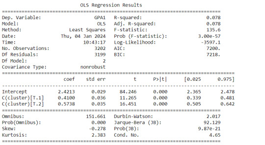
gpamod = smf.ols(formula='GPA1 ~ C(cluster)', data=sub1).fit() print (gpamod.summary())

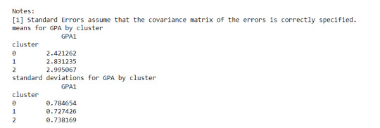
print ('means for GPA by cluster') m1= sub1.groupby('cluster').mean() print (m1)

print ('standard deviations for GPA by cluster') m2= sub1.groupby('cluster').std() print (m2)

Interpretation

The clustering average summary shows Cluster 0 has higher alcohol and marijuana problems, shows higher deviant and violent behavior, suffers from depression, has low self esteem,school connectedness, paraental and family connectedness. On the contrary, Cluster 2 shows the lowest alcohol and marijuana problems, lowest deviant & violent behavior,depression, and higher self esteem,school connectedness, paraental and family connectedness. Further, when validated against GPA score, we observe Cluster 0 shows the lowest average GPA and CLuster 2 has the highest average GPA which aligns with the summary statistics interpretation.

[courserabamarshall]

rom pandas import Series, DataFrame import pandas as pd import numpy as np import matplotlib.pylab as plt from sklearn.model_selection import train_test_split from sklearn import preprocessing from sklearn.cluster import KMeans

""" Data Management """ data = pd.read_csv("tree_addhealth")

upper-case all DataFrame column names

data.columns = map(str.upper, data.columns)

Data Management

data_clean = data.dropna()

subset clustering variables

cluster=data_clean[['ALCEVR1','MAREVER1','ALCPROBS1','DEVIANT1','VIOL1', 'DEP1','ESTEEM1','SCHCONN1','PARACTV', 'PARPRES','FAMCONCT']] cluster.describe()

standardize clustering variables to have mean=0 and sd=1

clustervar=cluster.copy() clustervar['ALCEVR1']=preprocessing.scale(clustervar['ALCEVR1'].astype('float64')) clustervar['ALCPROBS1']=preprocessing.scale(clustervar['ALCPROBS1'].astype('float64')) clustervar['MAREVER1']=preprocessing.scale(clustervar['MAREVER1'].astype('float64')) clustervar['DEP1']=preprocessing.scale(clustervar['DEP1'].astype('float64')) clustervar['ESTEEM1']=preprocessing.scale(clustervar['ESTEEM1'].astype('float64')) clustervar['VIOL1']=preprocessing.scale(clustervar['VIOL1'].astype('float64')) clustervar['DEVIANT1']=preprocessing.scale(clustervar['DEVIANT1'].astype('float64')) clustervar['FAMCONCT']=preprocessing.scale(clustervar['FAMCONCT'].astype('float64')) clustervar['SCHCONN1']=preprocessing.scale(clustervar['SCHCONN1'].astype('float64')) clustervar['PARACTV']=preprocessing.scale(clustervar['PARACTV'].astype('float64')) clustervar['PARPRES']=preprocessing.scale(clustervar['PARPRES'].astype('float64'))

split data into train and test sets

clus_train, clus_test = train_test_split(clustervar, test_size=.3, random_state=123)

k-means cluster analysis for 1-9 clusters

from scipy.spatial.distance import cdist clusters=range(1,10) meandist=[]

for k in clusters: model=KMeans(n_clusters=k) model.fit(clus_train) clusassign=model.predict(clus_train) meandist.append(sum(np.min(cdist(clus_train, model.cluster_centers_, 'euclidean'), axis=1)) / clus_train.shape[0])

""" Plot average distance from observations from the cluster centroid to use the Elbow Method to identify number of clusters to choose """

plt.plot(clusters, meandist) plt.xlabel('Number of clusters') plt.ylabel('Average distance') plt.title('Selecting k with the Elbow Method')

Interpret 3 cluster solution

model3=KMeans(n_clusters=3) model3.fit(clus_train) clusassign=model3.predict(clus_train)

plot clusters

from sklearn.decomposition import PCA pca_2 = PCA(2) plot_columns = pca_2.fit_transform(clus_train) plt.scatter(x=plot_columns[:,0], y=plot_columns[:,1], c=model3.labels_,) plt.xlabel('Canonical variable 1') plt.ylabel('Canonical variable 2') plt.title('Scatterplot of Canonical Variables for 3 Clusters') plt.show()

""" BEGIN multiple steps to merge cluster assignment with clustering variables to examine cluster variable means by cluster """

create a unique identifier variable from the index for the

cluster training data to merge with the cluster assignment variable

clus_train.reset_index(level=0, inplace=True)

create a list that has the new index variable

cluslist=list(clus_train['index'])

create a list of cluster assignments

labels=list(model3.labels_)

combine index variable list with cluster assignment list into a dictionary

newlist=dict(zip(cluslist, labels)) newlist

convert newlist dictionary to a dataframe

newclus=DataFrame.from_dict(newlist, orient='index') newclus

rename the cluster assignment column

newclus.columns = ['cluster']

now do the same for the cluster assignment variable

create a unique identifier variable from the index for the

cluster assignment dataframe

to merge with cluster training data

newclus.reset_index(level=0, inplace=True)

merge the cluster assignment dataframe with the cluster training variable dataframe

by the index variable

merged_train=pd.merge(clus_train, newclus, on='index') merged_train.head(n=100)

cluster frequencies

merged_train.cluster.value_counts()

""" END multiple steps to merge cluster assignment with clustering variables to examine cluster variable means by cluster """

FINALLY calculate clustering variable means by cluster

clustergrp = merged_train.groupby('cluster').mean() print ("Clustering variable means by cluster") print(clustergrp)

validate clusters in training data by examining cluster differences in GPA using ANOVA

first have to merge GPA with clustering variables and cluster assignment data

gpa_data=data_clean['GPA1']

split GPA data into train and test sets

gpa_train, gpa_test = train_test_split(gpa_data, test_size=.3, random_state=123) gpa_train1=pd.DataFrame(gpa_train) gpa_train1.reset_index(level=0, inplace=True) merged_train_all=pd.merge(gpa_train1, merged_train, on='index') sub1 = merged_train_all[['GPA1', 'cluster']].dropna()

import statsmodels.formula.api as smf import statsmodels.stats.multicomp as multi

gpamod = smf.ols(formula='GPA1 ~ C(cluster)', data=sub1).fit() print (gpamod.summary())

print ('means for GPA by cluster') m1= sub1.groupby('cluster').mean() print (m1)

print ('standard deviations for GPA by cluster') m2= sub1.groupby('cluster').std() print (m2)

mc1 = multi.MultiComparison(sub1['GPA1'], sub1['cluster']) res1 = mc1.tukeyhsd() print(res1.summary())

[astridchacon]

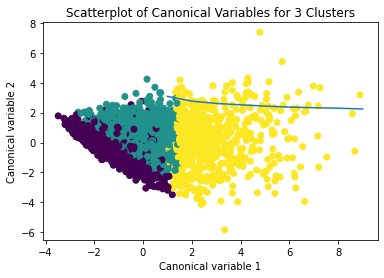
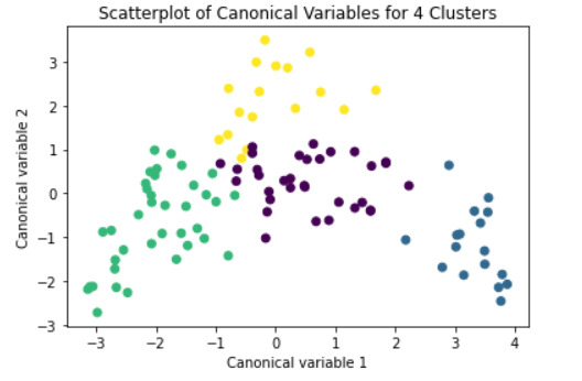
Machine Learning for Data Analysis - Week 4

#Load the data and convert the variables to numeric

import pandas as pd import numpy as np import matplotlib.pyplot as plt from sklearn.model_selection import train_test_split from sklearn.linear_model import LassoLarsCV import statsmodels.formula.api as smf import statsmodels.stats.multicomp as multi from sklearn import preprocessing from sklearn.cluster import KMeans

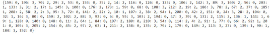
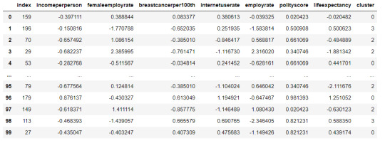
data = pd.read_csv('gapminder.csv', low_memory=False)

data['urbanrate'] = pd.to_numeric(data['urbanrate'], errors='coerce') data['incomeperperson'] = pd.to_numeric(data['incomeperperson'], errors='coerce') data['femaleemployrate'] = pd.to_numeric(data['femaleemployrate'], errors='coerce') data['breastcancerper100th'] = pd.to_numeric(data['breastcancerper100th'], errors='coerce') data['internetuserate'] = pd.to_numeric(data['internetuserate'], errors='coerce') data['employrate'] = pd.to_numeric(data['employrate'], errors='coerce') data['polityscore'] = pd.to_numeric(data['polityscore'], errors='coerce') data['lifeexpectancy'] = pd.to_numeric(data['lifeexpectancy'], errors='coerce')

sub1 = data.copy() data_clean = sub1.dropna()

#Subset the clustering variables

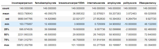
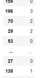
cluster = data_clean[['incomeperperson','femaleemployrate','breastcancerper100th','internetuserate', 'employrate', 'polityscore', 'lifeexpectancy']] cluster.describe()

#Standardize the clustering variables to have mean = 0 and standard deviation = 1

clustervar=cluster.copy() clustervar['incomeperperson']=preprocessing.scale(clustervar['incomeperperson'].astype('float64')) clustervar['femaleemployrate']=preprocessing.scale(clustervar['femaleemployrate'].astype('float64')) clustervar['breastcancerper100th']=preprocessing.scale(clustervar['breastcancerper100th'].astype('float64')) clustervar['internetuserate']=preprocessing.scale(clustervar['internetuserate'].astype('float64')) clustervar['employrate']=preprocessing.scale(clustervar['employrate'].astype('float64')) clustervar['polityscore']=preprocessing.scale(clustervar['polityscore'].astype('float64')) clustervar['lifeexpectancy']=preprocessing.scale(clustervar['lifeexpectancy'].astype('float64'))

#Split the data into train and test sets

clus_train, clus_test = train_test_split(clustervar, test_size=.3, random_state=123)

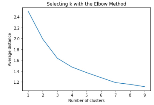
#Perform k-means cluster analysis for 1-9 clusters

from scipy.spatial.distance import cdist clusters = range(1,10) meandist = []

for k in clusters: model = KMeans(n_clusassign = k) model.fit(clus_train) clusters = model.predict(clus_train) meandist.append(sum(np.min(cdist(clus_train, model.cluster_centers_, 'euclidean'), axis=1)) / clus_train.shape[0])

#Plot average distance from observations from the cluster centroid to use the Elbow Method to identify number of clusters to choose

plt.plot(clusters, meandist) plt.xlabel('Number of clusters') plt.ylabel('Average distance') plt.title('Selecting k with the Elbow Method') plt.show()

#Interpret 3 cluster solution

model3 = KMeans(n_clusters=4) model3.fit(clus_train) clusassign = model3.predict(clus_train)

#Plot the clusters

from sklearn.decomposition import PCA pca_2 = PCA(2) plt.figure() plot_columns = pca_2.fit_transform(clus_train) plt.scatter(x=plot_columns[:,0], y=plot_columns[:,1], c=model3.labels_,) plt.xlabel('Canonical variable 1') plt.ylabel('Canonical variable 2') plt.title('Scatterplot of Canonical Variables for 4 Clusters') plt.show()

#Create a unique identifier variable from the index for the cluster training data to merge with the cluster assignment variable.

clus_train.reset_index(level=0, inplace=True)

#Create a list that has the new index variable

cluslist = list(clus_train['index'])

#Create a list of cluster assignments

labels = list(model3.labels_)

#Combine index variable list with cluster assignment list into a dictionary

newlist = dict(zip(cluslist, labels)) print(newlist)

#Convert newlist dictionary to a dataframe

newclus = pd.DataFrame.from_dict(newlist, orient='index')

#Rename the cluster assignment column

newclus.columns = ['cluster'] newclus

#Create a unique identifier variable from the index for the cluster assignment dataframe to merge with cluster training data

newclus.reset_index(level=0, inplace=True)

#Merge the cluster assignment dataframe with the cluster training variable dataframe by the index variable

merged_train = pd.merge(clus_train, newclus, on='index') merged_train.head(n=100)

#Cluster frequencies

merged_train.cluster.value_counts()

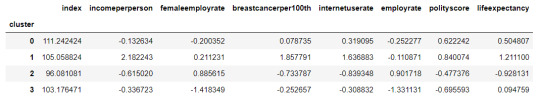
#Calculate clustering variable means by cluster

clustergrp = merged_train.groupby('cluster').mean() print ("Clustering variable means by cluster") clustergrp

#Validate clusters in training data by examining cluster differences in urbanrate using ANOVA.

#First, merge urbanrate with clustering variables and cluster assignment data

urbanrate_data = data_clean['urbanrate']

#Split urbanrate data into train and test sets

urbanrate_train, internetuserate_test = train_test_split(urbanrate_data, test_size=.3, random_state=123) urbanrate_train1=pd.DataFrame(urbanrate_train) urbanrate_train1.reset_index(level=0, inplace=True) merged_train_all=pd.merge(urbanrate_train1, merged_train, on='index') sub5 = merged_train_all[['urbanrate', 'cluster']].dropna() urbanrate_mod = smf.ols(formula='urbanrate ~ C(cluster)', data=sub5).fit() urbanrate_mod.summary()

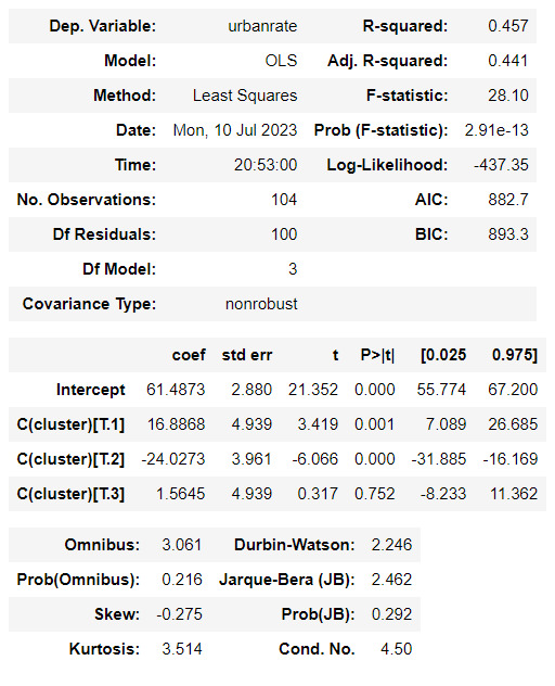
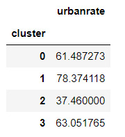
#Means for urbanrate by cluster

m1= sub5.groupby('cluster').mean() m1

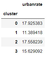
#Standard deviations for urbanrate by cluster

m2= sub5.groupby('cluster').std() m2

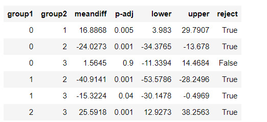
mc1 = multi.MultiComparison(sub5['urbanrate'], sub5['cluster']) res1 = mc1.tukeyhsd() res1.summary()

[archanawathore]

Data Management And Visualization - Assignment 4

Assignment 4 Python Code for Assignment 4 # -*- coding: utf-8 -*- """ Created on Wed Dec 23 15:49:41 2020 Assignment 4 @author: GB8PM0 """ #%% # import pandas and numpy import pandas import numpy import seaborn import matplotlib.pyplot as plt # any additional libraries would be imported here #Set PANDAS to show all columns in DataFrame pandas.set_option('display.max_columns', None) #Set PANDAS to show all rows in DataFrame pandas.set_option('display.max_rows', None) # bug fix for display formats to avoid run time errors pandas.set_option('display.float_format', lambda x:'%f'%x) #define data set to be used mydata = pandas.read_csv('addhealth_pds.csv', low_memory=False) #data management- create happiness types of 1 and2 don't get sad, 4 &5 get sad def happiness(row): if row['H1PF10'] == 1: return 1 elif row['H1PF10'] == 2 : return 1 elif row['H1PF10'] == 4 : return 0 elif row['H1PF10'] == 5 : return 0 mydata['happiness'] = mydata.apply (lambda row: happiness (row),axis=1) # Count of records in each option selected for happiness print("ph1 - % of happiness") ph1 = mydata["happiness"].value_counts(sort=True, normalize= True) * 100 print(ph1) # plot univariate graph of happiness seaborn.countplot(x="happiness", data=mydata) plt.xlabel('happiness') plt.title('happiness level') #%% #data management-creating satisfaction types of 1 and2 satisfied, 4 &5 Not Satisfied 3 neither def satisfaction(row): if row['H1PF5'] == 1: return 1 elif row['H1PF5'] == 2 : return 1 elif row['H1PF5'] == 4 : return 2 elif row['H1PF5'] == 5 : return 2 mydata['satisfaction'] = mydata.apply (lambda row: satisfaction (row),axis=1) # you can rename categorical variable values for graphing if original values are not informative # first change the variable format to categorical if you haven’t already done so mydata['satisfaction'] = mydata['satisfaction'] .astype('category') # second create a new variable that has the new variable value labels mydata['satisfaction'] =mydata['satisfaction'].cat.rename_categories(["Satisfied", "Not Satisfied"]) # % of records in each option selected for mother satifaction print("ps1 - % of satisfaction - Satisfaction with Mother") ps1 = mydata["satisfaction"].value_counts(sort=True, normalize=True) * 100 print(ps1) # plot univariate graph of satisfaction seaborn.countplot(x="satisfaction", data=mydata) plt.xlabel('Mother satisfaction') plt.title('Relationship with Mother satisfaction') #%% #data management-creating selfesteem types of 1 and2 good selfesteem, 4 &5 not good selfesteem def selfesteem(row): if row['H1PF33'] == 1: return 1 elif row['H1PF33'] == 2 : return 1 elif row['H1PF33'] == 4 : return 0 elif row['H1PF33'] == 5 : return 0 mydata['selfesteem'] = mydata.apply (lambda row: selfesteem (row),axis=1) # Count of records in each option selected for selfesteem print("% of selfesteem") pse1 = mydata["selfesteem"].value_counts(sort=True, normalize= True) print(pse1) # plot univariate graph of selfesteem seaborn.countplot(x="selfesteem", data=mydata) plt.xlabel('selfesteem') plt.title('selfesteem level') #plot bivariate bar graph C->C satisfaction and hapiness seaborn.catplot(x='satisfaction', y='happiness', data=mydata, kind="bar", ci=None) plt.xlabel('Relationship With Mother satisfaction') plt.ylabel('happiness') Variable 1 – happiness (H1PF10) Univariate graph of happiness. Created two groupings of “0” and “1”. 0 is for adolescents who felt sad and 1 is for adolescents who were not sad. 4435 of adolescents felt sadness, and 932 of adolescents were happy (not sad). Variable 2 – Satisfaction with Relation with Mother Created a Univariate graph of satisfaction with Mother relationship. Created two groupings of “Satisfied and “Not Satisfied”. Around 5404 adolescents were satisfied with the relationship with their mother, and around 363 were not satisfied with the relationship with their mother Variable 3 – Self Esteem Created two groupings of “0” and “1”. 0 is for adolescents who do not like themselves (have low self esteem), and 1 is for adolescents who like themselves (have high self esteem) . 5022 adolescents had high self esteem, and 592 had high self esteem Relationship with Mother Versus Happiness Created a bivariate graph between satisfaction with mother relationship to happiness. It looks like from the graph the 17.8% of adolescents who are satisfied with their relationship and are happy, whereas only 5% of adolescents who are not satisfied are happy

[mmm-plts]

Código K- means craters of mars

-- coding: utf-8 --

""" Created on Fri Jun 16 19:08:39 2023

@author: ANGELA """ from pandas import Series, DataFrame import pandas import numpy as np import matplotlib.pylab as plt from sklearn.model_selection import train_test_split from sklearn import preprocessing from sklearn.cluster import KMeans

"""Data management"""

data = pandas.read_csv('marscrater_pds.csv', low_memory=False) data['LATITUDE_CIRCLE_IMAGE']=pandas.to_numeric(data['LATITUDE_CIRCLE_IMAGE'],errors='coerce') data['LONGITUDE_CIRCLE_IMAGE']=pandas.to_numeric(data['LONGITUDE_CIRCLE_IMAGE'],errors='coerce') data['DIAM_CIRCLE_IMAGE']=pandas.to_numeric(data['DIAM_CIRCLE_IMAGE'],errors='coerce') data['NUMBER_LAYERS']=pandas.to_numeric(data['NUMBER_LAYERS'],errors='coerce') data['DEPTH_RIMFLOOR_TOPOG']=pandas.to_numeric(data['DEPTH_RIMFLOOR_TOPOG'],errors='coerce')

upper-case all DataFrame column names

data.columns = map(str.upper, data.columns) data_clean =data.dropna()

target = data_clean.DEPTH_RIMFLOOR_TOPOG

select predictor variables and target variable as separate data sets

cluster= data_clean[['LATITUDE_CIRCLE_IMAGE','LONGITUDE_CIRCLE_IMAGE','DIAM_CIRCLE_IMAGE']] cluster.describe()

standardize clustering variables to have mean=0 and sd=1

clustervar=cluster.copy() clustervar['LATITUDE_CIRCLE_IMAGE']=preprocessing.scale(clustervar['LATITUDE_CIRCLE_IMAGE'].astype('float64')) clustervar['LONGITUDE_CIRCLE_IMAGE']=preprocessing.scale(clustervar['LONGITUDE_CIRCLE_IMAGE'].astype('float64')) clustervar['DIAM_CIRCLE_IMAGE']=preprocessing.scale(clustervar['DIAM_CIRCLE_IMAGE'].astype('float64'))

clustervar['DEPTH_RIMFLOOR_TOPOG']=preprocessing.scale(clustervar['DEPTH_RIMFLOOR_TOPOG'].astype('float64'))

split data into train and test sets

clus_train, clus_test = train_test_split(clustervar, test_size=.3, random_state=200)

k-means cluster analysis for 1-9 clusters

from scipy.spatial.distance import cdist clusters=range(1,10) meandist=[]

Calculate cluster

for k in clusters: model=KMeans(n_clusters=k) model.fit(clus_train) clusassign=model.predict(clus_train) meandist.append(sum(np.min(cdist(clus_train, model.cluster_centers_, 'euclidean'), axis=1)) / clus_train.shape[0])

""" Plot average distance from observations from the cluster centroid to use the Elbow Method to identify number of clusters to choose """

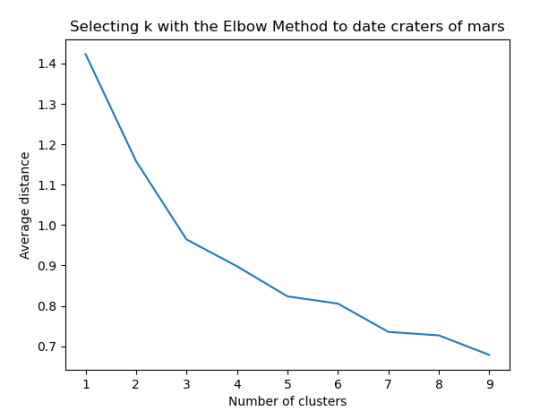
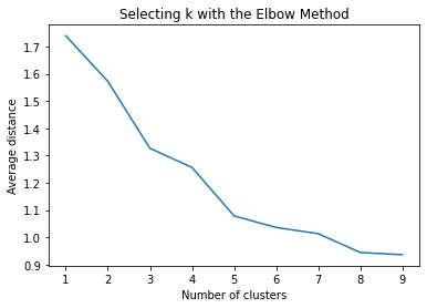
plt.plot(clusters, meandist) plt.xlabel('Number of clusters') plt.ylabel('Average distance') plt.title('Selecting k with the Elbow Method to date craters of mars')

Interpret 3 cluster solution

model3=KMeans(n_clusters=3) model3.fit(clus_train) clusassign=model3.predict(clus_train)

plot clusters

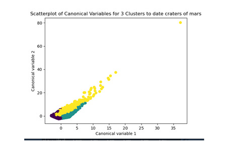
from sklearn.decomposition import PCA pca_2 = PCA(2) plot_columns = pca_2.fit_transform(clus_train) plt.scatter(x=plot_columns[:,0], y=plot_columns[:,1], c=model3.labels_,) plt.xlabel('Canonical variable 1') plt.ylabel('Canonical variable 2') plt.title('Scatterplot of Canonical Variables for 3 Clusters to date craters of mars') plt.show()

""" BEGIN multiple steps to merge cluster assignment with clustering variables to examine cluster variable means by cluster """

create a unique identifier variable from the index for the

cluster training data to merge with the cluster assignment variable

clus_train.reset_index(level=0, inplace=True)

create a list that has the new index variable

cluslist=list(clus_train['index'])

create a list of cluster assignments

labels=list(model3.labels_)

combine index variable list with cluster assignment list into a dictionary

newlist=dict(zip(cluslist, labels)) newlist

convert newlist dictionary to a dataframe

newclus=DataFrame.from_dict(newlist, orient='index') newclus

rename the cluster assignment column

newclus.columns = ['cluster']

now do the same for the cluster assignment variable

create a unique identifier variable from the index for the

cluster assignment dataframe

to merge with cluster training data

newclus.reset_index(level=0, inplace=True)

merge the cluster assignment dataframe with the cluster training variable dataframe

by the index variable

merged_train=pandas.merge(clus_train, newclus, on='index') merged_train.head(n=100)

cluster frequencies

merged_train.cluster.value_counts()

""" END multiple steps to merge cluster assignment with clustering variables to examine cluster variable means by cluster """

FINALLY calculate clustering variable means by cluster

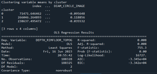
clustergrp = merged_train.groupby('cluster').mean() print ("Clustering variable means by cluster") print(clustergrp)

validate clusters in training data by examining cluster differences in DEPTH_RIMFLOOR_TOPOG using ANOVA

first have to merge DEPTH_RIMFLOOR_TOPOG with clustering variables and cluster assignment data

DRT_data=data_clean['DEPTH_RIMFLOOR_TOPOG']

split DEPTH_RIMFLOOR_TOPOG data into train and test sets

DRT_train, DRT_test = train_test_split(DRT_data, test_size=.3, random_state=123) DRT_train1=pandas.DataFrame(DRT_train) DRT_train1.reset_index(level=0, inplace=True) merged_train_all=pandas.merge(DRT_train1, merged_train, on='index') sub1 = merged_train_all[['DEPTH_RIMFLOOR_TOPOG', 'cluster']].dropna()

import statsmodels.formula.api as smf import statsmodels.stats.multicomp as multi

DTRmod = smf.ols(formula='DEPTH_RIMFLOOR_TOPOG ~ C(cluster)', data=sub1).fit() print (DTRmod.summary())

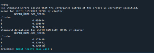
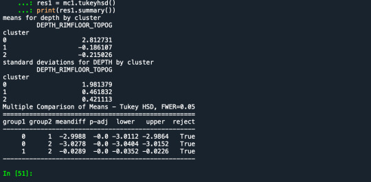
print ('means for DEPTH_RIMFLOOR_TOPOG by cluster') m1= sub1.groupby('cluster').mean() print (m1)

print ('standard deviations for DEPTH_RIMFLOOR_TOPOG by cluster') m2= sub1.groupby('cluster').std() print (m2)

mc1 = multi.MultiComparison(sub1['GPA1'], sub1['cluster']) res1 = mc1.tukeyhsd() print(res1.summary())

Resultados

Los cluster posibles son 3, 5, 7 y 8 donde se evidencia un punto de quiebre en la ilustración, por lo que se realizó la prueba con 3 clusters y se evidencia que puede presentarse un overfiting al esta muy cerca y cobre puestos los clusters

[hazrey-ab]

Data Management Decisions

STEP 1: Data Management Decisions

Coding out missing data: Identify how missing data is coded in your dataset and decide on a specific value to represent missing data. Let's say missing data is coded as "999" in your dataset, and you decide to recode it as "NA" to indicate missing values.

Coding in valid data: Ensure that valid data is appropriately coded and labeled in your dataset. Check if there are any inconsistencies or errors in the data coding and correct them if necessary.

Recoding variables: If needed, recode variables to align with your research question. For example, if you have a variable "Age" and want to create age groups, you can recode it into categories like "18-24," "25-34," "35-44," and so on.

Creating secondary variables: If there are specific calculations or derived variables that would be useful for your analysis, create them based on existing variables. For instance, if you have variables for height and weight, you can calculate the body mass index (BMI) as a secondary variable.

STEP 2: Running Frequency Distributions

Once you have implemented your data management decisions, you can proceed to run frequency distributions for your chosen variables. Ensure that your output is organized, labeled, and easy to interpret.

Here's an example program in Python to demonstrate the process:

import pandas as pd

Assuming you have a DataFrame called 'data' containing your variables

Code out missing data

data.replace(999, pd.NA, inplace=True)

Recode variables

data['Age_Group'] = pd.cut(data['Age'], bins=[18, 25, 35, 45, 55], labels=['18-24', '25-34', '35-44', '45-54'])

Create secondary variable

data['BMI'] = data['Weight'] / ((data['Height'] / 100) ** 2)

Frequency distribution for variable 'Gender'

gender_freq = data['Gender'].value_counts().reset_index().rename(columns={'index': 'Gender', 'Gender': 'Frequency'})

Frequency distribution for variable 'Age_Group'

age_group_freq = data['Age_Group'].value_counts().reset_index().rename(columns={'index': 'Age_Group', 'Age_Group': 'Frequency'})

Frequency distribution for variable 'BMI'

bmi_freq = data['BMI'].value_counts().reset_index().rename(columns={'index': 'BMI', 'BMI': 'Frequency'})

Print the frequency distributions

print("Frequency Distribution - Gender:") print(gender_freq) print()

print("Frequency Distribution - Age Group:") print(age_group_freq) print()

print("Frequency Distribution - BMI:") print(bmi_freq)

[win-n-nie]

MOD 4

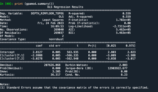
Results from the OLS regression results using the depth rim floor as the variable. the numbers appear to be close and now too far off. Cluster 0 having the biggest depth rim floor to the top.

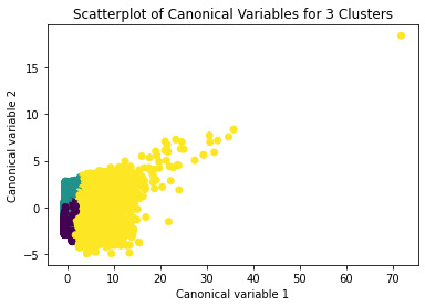
demonstrates that there is a giant overlap within the cluster groups however the yellow group appears to be more dispersed.

shows that theyre may be overlaps values 2, 3, 4, 5,6,7,8. This means that the variables being utilized are similar. Therefore the canonical variable test was performed to reduce the number of available variables.

CODE SCRIPT

from pandas import Series, DataFrame import pandas as pd import numpy as np import matplotlib.pylab as plt from sklearn.model_selection import train_test_split from sklearn import preprocessing from sklearn.cluster import KMeans

""" Data Management """ data = pd.read_csv('https://d3c33hcgiwev3.cloudfront.net/2c7ec69d0edd3b9599c0df80f0901a52_marscrater_pds.csv?Expires=1677369600&Signature=YDtfrRGhpLU3YbElRnuT3BynxPQdU1s3n6D-tR~Kb1tv7gDGdw2cKF49yGsmou3zWhP4ScXqbCGPbSdTd8SCPdZQpGXuj5B9I2lpUXObnn3OWFsNlQDz7WmrsngPFSdWHciEYCpCdYegyMmghimmDw1xZepgByZPuB5-Z6b3fOQ&Key-Pair-Id=APKAJLTNE6QMUY6HBC5A')

upper-case all DataFrame column names

data.columns = map(str.upper, data.columns)

Data Management

data_clean = data.dropna() data.dtypes

subset clustering variables

cluster=data_clean[['LATITUDE_CIRCLE_IMAGE','LONGITUDE_CIRCLE_IMAGE','DIAM_CIRCLE_IMAGE','DEPTH_RIMFLOOR_TOPOG', 'NUMBER_LAYERS']] cluster.describe()

standardize clustering variables to have mean=0 and sd=1

clustervar=cluster.copy() clustervar['LATITUDE_CIRCLE_IMAGE']=preprocessing.scale(clustervar['LATITUDE_CIRCLE_IMAGE'].astype('float64')) clustervar['LONGITUDE_CIRCLE_IMAGE']=preprocessing.scale(clustervar['LONGITUDE_CIRCLE_IMAGE'].astype('float64')) clustervar['DIAM_CIRCLE_IMAGE']=preprocessing.scale(clustervar['DIAM_CIRCLE_IMAGE'].astype('float64')) clustervar['DEPTH_RIMFLOOR_TOPOG']=preprocessing.scale(clustervar['DEPTH_RIMFLOOR_TOPOG'].astype('float64')) clustervar['NUMBER_LAYERS']=preprocessing.scale(clustervar['NUMBER_LAYERS'].astype('float64'))

split data into train and test sets

clus_train, clus_test = train_test_split(clustervar, test_size=.3, random_state=123)

k-means cluster analysis for 1-9 clusters

from scipy.spatial.distance import cdist clusters=range(1,10) meandist=[]

for k in clusters: model=KMeans(n_clusters=k) model.fit(clus_train) clusassign=model.predict(clus_train) meandist.append(sum(np.min(cdist(clus_train, model.cluster_centers_, 'euclidean'), axis=1)) / clus_train.shape[0])

""" Plot average distance from observations from the cluster centroid to use the Elbow Method to identify number of clusters to choose """

plt.plot(clusters, meandist) plt.xlabel('Number of clusters') plt.ylabel('Average distance') plt.title('Selecting k with the Elbow Method')

Interpret 3 cluster solution

model3=KMeans(n_clusters=3) model3.fit(clus_train) clusassign=model3.predict(clus_train)

plot clusters

from sklearn.decomposition import PCA pca_2 = PCA(2) plot_columns = pca_2.fit_transform(clus_train) plt.scatter(x=plot_columns[:,0], y=plot_columns[:,1], c=model3.labels_,) plt.xlabel('Canonical variable 1') plt.ylabel('Canonical variable 2') plt.title('Scatterplot of Canonical Variables for 3 Clusters') plt.show()

""" BEGIN multiple steps to merge cluster assignment with clustering variables to examine cluster variable means by cluster """

create a unique identifier variable from the index for the

cluster training data to merge with the cluster assignment variable

clus_train.reset_index(level=0, inplace=True)

create a list that has the new index variable

cluslist=list(clus_train['index'])

create a list of cluster assignments

labels=list(model3.labels_)

combine index variable list with cluster assignment list into a dictionary

newlist=dict(zip(cluslist, labels)) newlist

convert newlist dictionary to a dataframe

newclus=DataFrame.from_dict(newlist, orient='index') newclus

rename the cluster assignment column

newclus.columns = ['cluster']

now do the same for the cluster assignment variable

create a unique identifier variable from the index for the

cluster assignment dataframe

to merge with cluster training data

newclus.reset_index(level=0, inplace=True)

merge the cluster assignment dataframe with the cluster training variable dataframe

by the index variable

merged_train=pd.merge(clus_train, newclus, on='index') merged_train.head(n=100)

cluster frequencies

merged_train.cluster.value_counts()

""" END multiple steps to merge cluster assignment with clustering variables to examine cluster variable means by cluster """

FINALLY calculate clustering variable means by cluster

clustergrp = merged_train.groupby('cluster').mean() print ("Clustering variable means by cluster") print(clustergrp)

validate clusters in training data by examining cluster differences in GPA using ANOVA

first have to merge GPA with clustering variables and cluster assignment data

depth_data=data_clean['DEPTH_RIMFLOOR_TOPOG']

split GPA data into train and test sets

depth_train, depth_test = train_test_split(depth_data, test_size=.3, random_state=123) depth_train1=pd.DataFrame(layer_train) depth_train1.reset_index(level=0, inplace=True) merged_train_all=pd.merge(depth_train1, merged_train, on='index') sub1 = merged_train_all[['DEPTH_RIMFLOOR_TOPOG', 'cluster']].dropna()

import statsmodels.formula.api as smf import statsmodels.stats.multicomp as multi

gpamod = smf.ols(formula='DEPTH_RIMFLOOR_TOPOG ~ C(cluster)', data=sub1).fit() print (gpamod.summary())

print ('means for depth by cluster') m1= sub1.groupby('cluster').mean() print (m1)

print ('standard deviations for DEPTH by cluster') m2= sub1.groupby('cluster').std() print (m2)

mc1 = multi.MultiComparison(sub1['DEPTH_RIMFLOOR_TOPOG'], sub1['cluster']) res1 = mc1.tukeyhsd() print(res1.summary())

[monuonrise]

import pandas

import numpy

import scipy.stats

import seaborn

import matplotlib.pyplot as plt

nesarc = pandas.read_csv ('nesarc_pds.csv' , low_memory=False)

Set PANDAS to show all columns in DataFrame

pandas.set_option('display.max_columns', None)

#Set PANDAS to show all rows in DataFrame

pandas.set_option('display.max_rows', None)

nesarc.columns = map(str.upper , nesarc.columns)

pandas.set_option('display.float_format' , lambda x:'%f'%x)

#Change my variables to numeric

nesarc['AGE'] = pandas.to_numeric(nesarc['AGE'], errors='coerce') nesarc['S3BQ4'] = pandas.to_numeric(nesarc['S3BQ4'], errors='coerce') nesarc['S3BQ1A5'] = pandas.to_numeric(nesarc['S3BQ1A5'], errors='coerce') nesarc['S3BD5Q2B'] = pandas.to_numeric(nesarc['S3BD5Q2B'], errors='coerce') nesarc['S3BD5Q2E'] = pandas.to_numeric(nesarc['S3BD5Q2E'], errors='coerce') nesarc['MAJORDEP12'] = pandas.to_numeric(nesarc['MAJORDEP12'], errors='coerce') nesarc['GENAXDX12'] = pandas.to_numeric(nesarc['GENAXDX12'], errors='coerce')

#Subset my sample

subset1 = nesarc[(nesarc['AGE']>=18) & (nesarc['AGE']<=30)] # Ages 18-30 subsetc1 = subset1.copy()

subset2 = nesarc[(nesarc['AGE']>=18) & (nesarc['AGE']<=30) & (nesarc['S3BQ1A5']==1)] # Cannabis users, ages 18-30 subsetc2 = subset2.copy()

#Setting missing data for frequency and cannabis use, variables S3BD5Q2E, S3BQ1A5

subsetc1['S3BQ1A5']=subsetc1['S3BQ1A5'].replace(9, numpy.nan) subsetc2['S3BD5Q2E']=subsetc2['S3BD5Q2E'].replace('BL', numpy.nan) subsetc2['S3BD5Q2E']=subsetc2['S3BD5Q2E'].replace(99, numpy.nan)

Contingency table of observed counts of major depression diagnosis (response variable) within cannabis use (explanatory variable), in ages 18-30

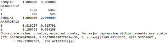
contab1=pandas.crosstab(subsetc1['MAJORDEP12'], subsetc1['S3BQ1A5']) print (contab1)

#Column percentages

colsum=contab1.sum(axis=0) colpcontab=contab1/colsum print(colpcontab)

#Chi-square calculations for major depression within cannabis use status

print ('Chi-square value, p value, expected counts, for major depression within cannabis use status') chsq1= scipy.stats.chi2_contingency(contab1) print (chsq1)

#Contingency table of observed counts of geberal anxiety diagnosis (response variable) within cannabis use (explanatory variable), in ages 18-30

contab2=pandas.crosstab(subsetc1['GENAXDX12'], subsetc1['S3BQ1A5']) print (contab2)

#Column percentages

colsum2=contab2.sum(axis=0) colpcontab2=contab2/colsum2 print(colpcontab2)

#Chi-square calculations for general anxiety within cannabis use status

print ('Chi-square value, p value, expected counts, for general anxiety within cannabis use status') chsq2= scipy.stats.chi2_contingency(contab2) print (chsq2)

#

#Contingency table of observed counts of major depression diagnosis (response variable) within frequency of cannabis use (10 level explanatory variable), in ages 18-30

contab3=pandas.crosstab(subset2['MAJORDEP12'], subset2['S3BD5Q2E']) print (contab3)

#Column percentages

colsum3=contab3.sum(axis=0) colpcontab3=contab3/colsum3 print(colpcontab3)

#Chi-square calculations for mahor depression within frequency of cannabis use groups

print ('Chi-square value, p value, expected counts for major depression associated frequency of cannabis use') chsq3= scipy.stats.chi2_contingency(contab3) print (chsq3)

recode1 = {1: 9, 2: 8, 3: 7, 4: 6, 5: 5, 6: 4, 7: 3, 8: 2, 9: 1} # Dictionary with details of frequency variable reverse-recode subsetc2['CUFREQ'] = subsetc2['S3BD5Q2E'].map(recode1) # Change variable name from S3BD5Q2E to CUFREQ

subsetc2["CUFREQ"] = subsetc2["CUFREQ"].astype('category')

#Rename graph labels for better interpretation

subsetc2['CUFREQ'] = subsetc2['CUFREQ'].cat.rename_categories(["2 times/year","3-6 times/year","7-11 times/years","Once a month","2-3 times/month","1-2 times/week","3-4 times/week","Nearly every day","Every day"])

#Graph percentages of major depression within each cannabis smoking frequency group

plt.figure(figsize=(12,4)) # Change plot size ax1 = seaborn.factorplot(x="CUFREQ", y="MAJORDEP12", data=subsetc2, kind="bar", ci=None) ax1.set_xticklabels(rotation=40, ha="right") # X-axis labels rotation plt.xlabel('Frequency of cannabis use') plt.ylabel('Proportion of Major Depression') plt.show()

#Post hoc test, pair comparison of frequency groups 1 and 9, 'Every day' and '2 times a year'

recode2 = {1: 1, 9: 9} subsetc2['COMP1v9']= subsetc2['S3BD5Q2E'].map(recode2)

#Contingency table of observed counts

ct4=pandas.crosstab(subsetc2['MAJORDEP12'], subsetc2['COMP1v9']) print (ct4)

#Column percentages

colsum4=ct4.sum(axis=0) colpcontab4=ct4/colsum4 print(colpcontab4)

#Chi-square calculations for pair comparison of frequency groups 1 and 9, 'Every day' and '2 times a year'

print ('Chi-square value, p value, expected counts, for pair comparison of frequency groups -Every day- and -2 times a year-') cs4= scipy.stats.chi2_contingency(ct4) print (cs4)

#Post hoc test, pair comparison of frequency groups 2 and 6, 'Nearly every day' and 'Once a month'

recode3 = {2: 2, 6: 6} subsetc2['COMP2v6']= subsetc2['S3BD5Q2E'].map(recode3)

#Contingency table of observed counts

ct5=pandas.crosstab(subsetc2['MAJORDEP12'], subsetc2['COMP2v6']) print (ct5)

#Column percentages

colsum5=ct5.sum(axis=0) colpcontab5=ct5/colsum5 print(colpcontab5)

#Chi-square calculations for pair comparison of frequency groups 2 and 6, 'Nearly every day' and 'Once a month'

print ('Chi-square value, p value, expected counts for pair comparison of frequency groups -Nearly every day- and -Once a month-') cs5= scipy.stats.chi2_contingency(ct5) print (cs5)

[taj-15]

Running a Chi-Square Test of Independence for my data

import pandas import numpy import scipy.stats import seaborn import matplotlib.pyplot as plt

nesarc = pandas.read_csv ('nesarc_pds.csv' , low_memory=False)

Set PANDAS to show all columns in DataFrame

pandas.set_option('display.max_columns', None)

#Set PANDAS to show all rows in DataFrame

pandas.set_option('display.max_rows', None)

nesarc.columns = map(str.upper , nesarc.columns)

pandas.set_option('display.float_format' , lambda x:'%f'%x)

#Change my variables to numeric

nesarc['AGE'] = pandas.to_numeric(nesarc['AGE'], errors='coerce') nesarc['S3BQ4'] = pandas.to_numeric(nesarc['S3BQ4'], errors='coerce') nesarc['S3BQ1A5'] = pandas.to_numeric(nesarc['S3BQ1A5'], errors='coerce') nesarc['S3BD5Q2B'] = pandas.to_numeric(nesarc['S3BD5Q2B'], errors='coerce') nesarc['S3BD5Q2E'] = pandas.to_numeric(nesarc['S3BD5Q2E'], errors='coerce') nesarc['MAJORDEP12'] = pandas.to_numeric(nesarc['MAJORDEP12'], errors='coerce') nesarc['GENAXDX12'] = pandas.to_numeric(nesarc['GENAXDX12'], errors='coerce')

#Subset my sample

subset1 = nesarc[(nesarc['AGE']>=18) & (nesarc['AGE']<=30)] # Ages 18-30 subsetc1 = subset1.copy()

subset2 = nesarc[(nesarc['AGE']>=18) & (nesarc['AGE']<=30) & (nesarc['S3BQ1A5']==1)] # Cannabis users, ages 18-30 subsetc2 = subset2.copy()

#Setting missing data for frequency and cannabis use, variables S3BD5Q2E, S3BQ1A5

subsetc1['S3BQ1A5']=subsetc1['S3BQ1A5'].replace(9, numpy.nan) subsetc2['S3BD5Q2E']=subsetc2['S3BD5Q2E'].replace('BL', numpy.nan) subsetc2['S3BD5Q2E']=subsetc2['S3BD5Q2E'].replace(99, numpy.nan)

Contingency table of observed counts of major depression diagnosis (response variable) within cannabis use (explanatory variable), in ages 18-30

contab1=pandas.crosstab(subsetc1['MAJORDEP12'], subsetc1['S3BQ1A5']) print (contab1)

#Column percentages

colsum=contab1.sum(axis=0) colpcontab=contab1/colsum print(colpcontab)

#Chi-square calculations for major depression within cannabis use status

print ('Chi-square value, p value, expected counts, for major depression within cannabis use status') chsq1= scipy.stats.chi2_contingency(contab1) print (chsq1)

#Contingency table of observed counts of geberal anxiety diagnosis (response variable) within cannabis use (explanatory variable), in ages 18-30

contab2=pandas.crosstab(subsetc1['GENAXDX12'], subsetc1['S3BQ1A5']) print (contab2)

#Column percentages

colsum2=contab2.sum(axis=0) colpcontab2=contab2/colsum2 print(colpcontab2)

#Chi-square calculations for general anxiety within cannabis use status

print ('Chi-square value, p value, expected counts, for general anxiety within cannabis use status') chsq2= scipy.stats.chi2_contingency(contab2) print (chsq2)

#

#Contingency table of observed counts of major depression diagnosis (response variable) within frequency of cannabis use (10 level explanatory variable), in ages 18-30

contab3=pandas.crosstab(subset2['MAJORDEP12'], subset2['S3BD5Q2E']) print (contab3)

#Column percentages

colsum3=contab3.sum(axis=0) colpcontab3=contab3/colsum3 print(colpcontab3)

#Chi-square calculations for mahor depression within frequency of cannabis use groups

print ('Chi-square value, p value, expected counts for major depression associated frequency of cannabis use') chsq3= scipy.stats.chi2_contingency(contab3) print (chsq3)

recode1 = {1: 9, 2: 8, 3: 7, 4: 6, 5: 5, 6: 4, 7: 3, 8: 2, 9: 1} # Dictionary with details of frequency variable reverse-recode subsetc2['CUFREQ'] = subsetc2['S3BD5Q2E'].map(recode1) # Change variable name from S3BD5Q2E to CUFREQ

subsetc2["CUFREQ"] = subsetc2["CUFREQ"].astype('category')

#Rename graph labels for better interpretation

subsetc2['CUFREQ'] = subsetc2['CUFREQ'].cat.rename_categories(["2 times/year","3-6 times/year","7-11 times/years","Once a month","2-3 times/month","1-2 times/week","3-4 times/week","Nearly every day","Every day"])

#Graph percentages of major depression within each cannabis smoking frequency group

plt.figure(figsize=(12,4)) # Change plot size ax1 = seaborn.factorplot(x="CUFREQ", y="MAJORDEP12", data=subsetc2, kind="bar", ci=None) ax1.set_xticklabels(rotation=40, ha="right") # X-axis labels rotation plt.xlabel('Frequency of cannabis use') plt.ylabel('Proportion of Major Depression') plt.show()

#Post hoc test, pair comparison of frequency groups 1 and 9, 'Every day' and '2 times a year'

recode2 = {1: 1, 9: 9} subsetc2['COMP1v9']= subsetc2['S3BD5Q2E'].map(recode2)

#Contingency table of observed counts

ct4=pandas.crosstab(subsetc2['MAJORDEP12'], subsetc2['COMP1v9']) print (ct4)

#Column percentages

colsum4=ct4.sum(axis=0) colpcontab4=ct4/colsum4 print(colpcontab4)

#Chi-square calculations for pair comparison of frequency groups 1 and 9, 'Every day' and '2 times a year'

print ('Chi-square value, p value, expected counts, for pair comparison of frequency groups -Every day- and -2 times a year-') cs4= scipy.stats.chi2_contingency(ct4) print (cs4)

#Post hoc test, pair comparison of frequency groups 2 and 6, 'Nearly every day' and 'Once a month'

recode3 = {2: 2, 6: 6} subsetc2['COMP2v6']= subsetc2['S3BD5Q2E'].map(recode3)

#Contingency table of observed counts

ct5=pandas.crosstab(subsetc2['MAJORDEP12'], subsetc2['COMP2v6']) print (ct5)

#Column percentages

colsum5=ct5.sum(axis=0) colpcontab5=ct5/colsum5 print(colpcontab5)

#Chi-square calculations for pair comparison of frequency groups 2 and 6, 'Nearly every day' and 'Once a month'

print ('Chi-square value, p value, expected counts for pair comparison of frequency groups -Nearly every day- and -Once a month-') cs5= scipy.stats.chi2_contingency(ct5) print (cs5)