#create dataframe from dictionary in pandas
Explore tagged Tumblr posts
Visit Tumblr Blog
Explore Tumblr blogs with no restrictions, modern design and the best experience.
Last Seen Tumblr Blogs


Fun Fact
The most popular pages on Tumblr are about Minecraft, GIFs, and David J. Peterson.
Text
DataFrame in Pandas: Guide to Creating Awesome DataFrames
Explore how to create a dataframe in Pandas, including data input methods, customization options, and practical examples.
Data analysis used to be a daunting task, reserved for statisticians and mathematicians. But with the rise of powerful tools like Python and its fantastic library, Pandas, anyone can become a data whiz! Pandas, in particular, shines with its DataFrames, these nifty tables that organize and manipulate data like magic. But where do you start? Fear not, fellow data enthusiast, for this guide will…
View On WordPress
#advanced dataframe features#aggregating data in pandas#create dataframe from dictionary in pandas#create dataframe from list in pandas#create dataframe in pandas#data manipulation in pandas#dataframe indexing#filter dataframe by condition#filter dataframe by multiple conditions#filtering data in pandas#grouping data in pandas#how to make a dataframe in pandas#manipulating data in pandas#merging dataframes#pandas data structures#pandas dataframe tutorial#python dataframe basics#rename columns in pandas dataframe#replace values in pandas dataframe#select columns in pandas dataframe#select rows in pandas dataframe#set column names in pandas dataframe#set row names in pandas dataframe
0 notes
Text
Pandas DataFrame Tutorial: Ways to Create and Manipulate Data in Python Are you diving into data analysis with Python? Then you're about to become best friends with pandas DataFrames. These powerful, table-like structures are the backbone of data manipulation in Python, and knowing how to create them is your first step toward becoming a data analysis expert. In this comprehensive guide, we'll explore everything you need to know about creating pandas DataFrames, from basic methods to advanced techniques. Whether you're a beginner or looking to level up your skills, this tutorial has got you covered. Getting Started with Pandas Before we dive in, let's make sure you have everything set up. First, you'll need to install pandas if you haven't already: pythonCopypip install pandas Then, import pandas in your Python script: pythonCopyimport pandas as pd 1. Creating a DataFrame from Lists The simplest way to create a DataFrame is using Python lists. Here's how: pythonCopy# Creating a basic DataFrame from lists data = 'name': ['John', 'Emma', 'Alex', 'Sarah'], 'age': [28, 24, 32, 27], 'city': ['New York', 'London', 'Paris', 'Tokyo'] df = pd.DataFrame(data) print(df) This creates a clean, organized table with your data. The keys in your dictionary become column names, and the values become the data in each column. 2. Creating a DataFrame from NumPy Arrays When working with numerical data, NumPy arrays are your friends: pythonCopyimport numpy as np # Creating a DataFrame from a NumPy array array_data = np.random.rand(4, 3) df_numpy = pd.DataFrame(array_data, columns=['A', 'B', 'C'], index=['Row1', 'Row2', 'Row3', 'Row4']) print(df_numpy) 3. Reading Data from External Sources Real-world data often comes from files. Here's how to create DataFrames from different file formats: pythonCopy# CSV files df_csv = pd.read_csv('your_file.csv') # Excel files df_excel = pd.read_excel('your_file.xlsx') # JSON files df_json = pd.read_json('your_file.json') 4. Creating a DataFrame from a List of Dictionaries Sometimes your data comes as a list of dictionaries, especially when working with APIs: pythonCopy# List of dictionaries records = [ 'name': 'John', 'age': 28, 'department': 'IT', 'name': 'Emma', 'age': 24, 'department': 'HR', 'name': 'Alex', 'age': 32, 'department': 'Finance' ] df_records = pd.DataFrame(records) print(df_records) 5. Creating an Empty DataFrame Sometimes you need to start with an empty DataFrame and fill it later: pythonCopy# Create an empty DataFrame with defined columns columns = ['Name', 'Age', 'City'] df_empty = pd.DataFrame(columns=columns) # Add data later new_row = 'Name': 'Lisa', 'Age': 29, 'City': 'Berlin' df_empty = df_empty.append(new_row, ignore_index=True) 6. Advanced DataFrame Creation Techniques Using Multi-level Indexes pythonCopy# Creating a DataFrame with multi-level index arrays = [ ['2023', '2023', '2024', '2024'], ['Q1', 'Q2', 'Q1', 'Q2'] ] data = 'Sales': [100, 120, 150, 180] df_multi = pd.DataFrame(data, index=arrays) print(df_multi) Creating Time Series DataFrames pythonCopy# Creating a time series DataFrame dates = pd.date_range('2024-01-01', periods=6, freq='D') df_time = pd.DataFrame(np.random.randn(6, 4), index=dates, columns=['A', 'B', 'C', 'D']) Best Practices and Tips Always Check Your Data Types pythonCopy# Check data types of your DataFrame print(df.dtypes) Set Column Names Appropriately Use clear, descriptive column names without spaces: pythonCopydf.columns = ['first_name', 'last_name', 'email'] Handle Missing Data pythonCopy# Check for missing values print(df.isnull().sum()) # Fill missing values df.fillna(0, inplace=True) Common Pitfalls to Avoid Memory Management: Be cautious with large datasets. Use appropriate data types to minimize memory usage:
pythonCopy# Optimize numeric columns df['integer_column'] = df['integer_column'].astype('int32') Copy vs. View: Understand when you're creating a copy or a view: pythonCopy# Create a true copy df_copy = df.copy() Conclusion Creating pandas DataFrames is a fundamental skill for any data analyst or scientist working with Python. Whether you're working with simple lists, complex APIs, or external files, pandas provides flexible and powerful ways to structure your data. Remember to: Choose the most appropriate method based on your data source Pay attention to data types and memory usage Use clear, consistent naming conventions Handle missing data appropriately With these techniques in your toolkit, you're well-equipped to handle any data manipulation task that comes your way. Practice with different methods and explore the pandas documentation for more advanced features as you continue your data analysis journey. Additional Resources Official pandas documentation Pandas cheat sheet Python for Data Science Handbook Real-world pandas examples on GitHub Now you're ready to start creating and manipulating DataFrames like a pro. Happy coding!
0 notes
Text
Level Up Data Science Skills with Python: A Full Guide
Data science is one of the most in-demand careers in the world today, and Python is its go-to language. Whether you're just starting out or looking to sharpen your skills, mastering Python can open doors to countless opportunities in data analytics, machine learning, artificial intelligence, and beyond.
In this guide, we’ll explore how Python can take your data science abilities to the next level—covering core concepts, essential libraries, and practical tips for real-world application.
Why Python for Data Science?
Python’s popularity in data science is no accident. It’s beginner-friendly, versatile, and has a massive ecosystem of libraries and tools tailored specifically for data work. Here's why it stands out:
Clear syntax simplifies learning and ensures easier maintenance.
Community support means constant updates and rich documentation.
Powerful libraries for everything from data manipulation to visualization and machine learning.
Core Python Concepts Every Data Scientist Should Know
Establish a solid base by thoroughly understanding the basics before advancing to more complex methods:
Variables and Data Types: Get familiar with strings, integers, floats, lists, and dictionaries.
Control Flow: Master if-else conditions, for/while loops, and list comprehensions through practice.
Functions and Modules: Understand how to create reusable code by defining functions.
File Handling: Leverage built-in functions to handle reading from and writing to files.
Error Handling: Use try-except blocks to write robust programs.
Mastering these foundations ensures you can write clean, efficient code—critical for working with complex datasets.
Must-Know Python Libraries for Data Science
Once you're confident with Python basics, it’s time to explore the libraries that make data science truly powerful:
NumPy: For numerical operations and array manipulation. It forms the essential foundation for a wide range of data science libraries.
Pandas: Used for data cleaning, transformation, and analysis. DataFrames are essential for handling structured data.
Matplotlib & Seaborn: These libraries help visualize data. While Matplotlib gives you control, Seaborn makes it easier with beautiful default styles.
Scikit-learn: Perfect for building machine learning models. Features algorithms for tasks like classification, regression, clustering, and additional methods.
TensorFlow & PyTorch: For deep learning and neural networks. Choose one based on your project needs and personal preference.
Real-World Projects to Practice
Applying what you’ve learned through real-world projects is key to skill development. Here are a few ideas:
Data Cleaning Challenge: Work with messy datasets and clean them using Pandas.
Exploratory Data Analysis (EDA): Analyze a dataset, find patterns, and visualize results.
Build a Machine Learning Model: Use Scikit-learn to create a prediction model for housing prices, customer churn, or loan approval.
Sentiment Analysis: Use natural language processing (NLP) to analyze product reviews or tweets.
Completing these projects can enhance your portfolio and attract the attention of future employers.
Tips to Accelerate Your Learning
Join online courses and bootcamps: Join Online Platforms
Follow open-source projects on GitHub: Contribute to or learn from real codebases.
Engage with the community: Join forums like Stack Overflow or Reddit’s r/datascience.
Read documentation and blogs: Keep yourself informed about new features and optimal practices.
Set goals and stay consistent: Data science is a long-term journey, not a quick race.
Python is the cornerstone of modern data science. Whether you're manipulating data, building models, or visualizing insights, Python equips you with the tools to succeed. By mastering its fundamentals and exploring its powerful libraries, you can confidently tackle real-world data challenges and elevate your career in the process. If you're looking to sharpen your skills, enrolling in a Python course in Gurgaon can be a great way to get expert guidance and hands-on experience.
DataMites Institute stands out as a top international institute providing in-depth education in data science, AI, and machine learning. We provide expert-led courses designed for both beginners and professionals aiming to boost their careers.
Python vs R - What is the Difference, Pros and Cons
youtube
#python course#python training#python institute#learnpython#python#pythoncourseingurgaon#pythoncourseinindia#Youtube
0 notes
Text
K-mean Analysis
Script:
from pandas import Series, DataFrame import pandas as pd import numpy as np import matplotlib.pylab as plt from sklearn.model_selection import train_test_split from sklearn import preprocessing from sklearn.cluster import KMeans import os """ Data Management """
data = pd.read_csv("tree_addhealth.csv")
upper-case all DataFrame column names
data.columns = map(str.upper, data.columns)
Data Management
data_clean = data.dropna()
subset clustering variables
cluster=data_clean[['ALCEVR1','MAREVER1','ALCPROBS1','DEVIANT1','VIOL1', 'DEP1','ESTEEM1','SCHCONN1','PARACTV', 'PARPRES','FAMCONCT']] cluster.describe()
standardize clustering variables to have mean=0 and sd=1
clustervar=cluster.copy() clustervar['ALCEVR1']=preprocessing.scale(clustervar['ALCEVR1'].astype('float64')) clustervar['ALCPROBS1']=preprocessing.scale(clustervar['ALCPROBS1'].astype('float64')) clustervar['MAREVER1']=preprocessing.scale(clustervar['MAREVER1'].astype('float64')) clustervar['DEP1']=preprocessing.scale(clustervar['DEP1'].astype('float64')) clustervar['ESTEEM1']=preprocessing.scale(clustervar['ESTEEM1'].astype('float64')) clustervar['VIOL1']=preprocessing.scale(clustervar['VIOL1'].astype('float64')) clustervar['DEVIANT1']=preprocessing.scale(clustervar['DEVIANT1'].astype('float64')) clustervar['FAMCONCT']=preprocessing.scale(clustervar['FAMCONCT'].astype('float64')) clustervar['SCHCONN1']=preprocessing.scale(clustervar['SCHCONN1'].astype('float64')) clustervar['PARACTV']=preprocessing.scale(clustervar['PARACTV'].astype('float64')) clustervar['PARPRES']=preprocessing.scale(clustervar['PARPRES'].astype('float64'))
split data into train and test sets
clus_train, clus_test = train_test_split(clustervar, test_size=.3, random_state=123)
k-means cluster analysis for 1-9 clusters
from scipy.spatial.distance import cdist clusters=range(1,9) meandist=[]
for k in clusters: model=KMeans(n_clusters=k) model.fit(clus_train) clusassign=model.predict(clus_train) meandist.append(sum(np.min(cdist(clus_train, model.cluster_centers_, 'euclidean'), axis=1)) / clus_train.shape[0])
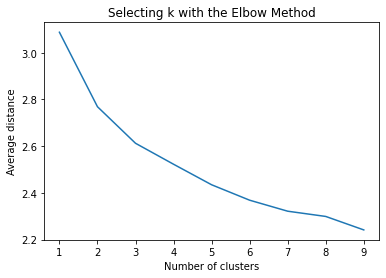
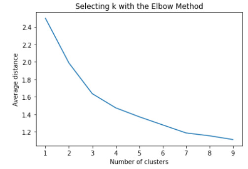
""" Plot average distance from observations from the cluster centroid to use the Elbow Method to identify number of clusters to choose """
plt.plot(clusters, meandist) plt.xlabel('Number of clusters') plt.ylabel('Average distance') plt.title('Selecting k with the Elbow Method')
Interpret 3 cluster solution
model3=KMeans(n_clusters=2) model3.fit(clus_train) clusassign=model3.predict(clus_train)
plot clusters
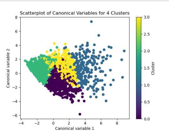
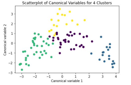
from sklearn.decomposition import PCA pca_2 = PCA(2) plot_columns = pca_2.fit_transform(clus_train) plt.scatter(x=plot_columns[:,0], y=plot_columns[:,1], c=model3.labels_) plt.xlabel('Canonical variable 1') plt.ylabel('Canonical variable 2') plt.title('Scatterplot of Canonical Variables for 4 Clusters')
Add the legend to the plot
import matplotlib.patches as mpatches patches = [mpatches.Patch(color=plt.cm.viridis(i/4), label=f'Cluster {i}') for i in range(4)]
plt.legend(handles=patches, title="Clusters") plt.show()
""" BEGIN multiple steps to merge cluster assignment with clustering variables to examine cluster variable means by cluster """
create a unique identifier variable from the index for the
cluster training data to merge with the cluster assignment variable
clus_train.reset_index(level=0, inplace=True)
create a list that has the new index variable
cluslist=list(clus_train['index'])
create a list of cluster assignments
labels=list(model3.labels_)
combine index variable list with cluster assignment list into a dictionary
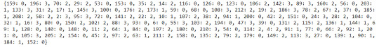
newlist=dict(zip(cluslist, labels)) newlist
convert newlist dictionary to a dataframe
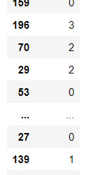
newclus=DataFrame.from_dict(newlist, orient='index') newclus
rename the cluster assignment column
newclus.columns = ['cluster']
now do the same for the cluster assignment variable
create a unique identifier variable from the index for the
cluster assignment dataframe
to merge with cluster training data
newclus.reset_index(level=0, inplace=True)
merge the cluster assignment dataframe with the cluster training variable dataframe
by the index variable
merged_train=pd.merge(clus_train, newclus, on='index') merged_train.head(n=100)
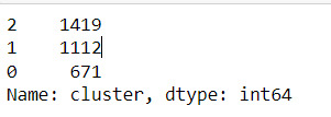
cluster frequencies
merged_train.cluster.value_counts()
""" END multiple steps to merge cluster assignment with clustering variables to examine cluster variable means by cluster """
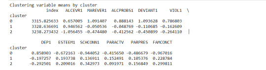
FINALLY calculate clustering variable means by cluster
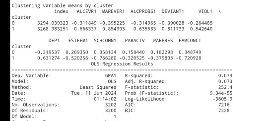
clustergrp = merged_train.groupby('cluster').mean() print ("Clustering variable means by cluster") print(clustergrp)
validate clusters in training data by examining cluster differences in GPA using ANOVA
first have to merge GPA with clustering variables and cluster assignment data
gpa_data=data_clean['GPA1']
split GPA data into train and test sets
gpa_train, gpa_test = train_test_split(gpa_data, test_size=.3, random_state=123) gpa_train1=pd.DataFrame(gpa_train) gpa_train1.reset_index(level=0, inplace=True) merged_train_all=pd.merge(gpa_train1, merged_train, on='index') sub1 = merged_train_all[['GPA1', 'cluster']].dropna()
import statsmodels.formula.api as smf import statsmodels.stats.multicomp as multi
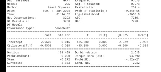
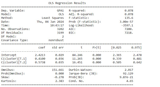
gpamod = smf.ols(formula='GPA1 ~ C(cluster)', data=sub1).fit() print (gpamod.summary())
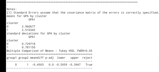
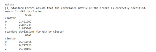
print ('means for GPA by cluster') m1= sub1.groupby('cluster').mean() print (m1)
print ('standard deviations for GPA by cluster') m2= sub1.groupby('cluster').std() print (m2)
mc1 = multi.MultiComparison(sub1['GPA1'], sub1['cluster']) res1 = mc1.tukeyhsd() print(res1.summary())
------------------------------------------------------------------------------
PLOTS:

------------------------------------------------------------------------------ANALYSING:
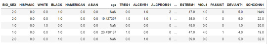
The K-mean cluster analysis is trying to identify subgroups of adolescents based on their similarity using the following 11 variables:
(Binary variables)
ALCEVR1 = ever used alcohol
MAREVER1 = ever used marijuana
(Quantitative variables)
ALCPROBS1 = Alcohol problem
DEVIANT1 = behaviors scale
VIOL1 = Violence scale
DEP1 = depression scale
ESTEEM1 = Self-esteem
SCHCONN1= School connectiveness
PARACTV = parent activities
PARPRES = parent presence
FAMCONCT = family connectiveness
The test was split with 70% for the training set and 30% for the test set. 9 clusters were conducted and the results are shown the plot 1. The plot suggest 2,4 , 5 and 6 solutions might be interpreted.
The second plot shows the canonical discriminant analyses of the 4 cluster solutions. Clusters 0 and 3 are very densely packed together with relatively low within-cluster variance whereas clusters 1 and 2 were spread out more than the other clusters, especially cluster 1 which means there is higher variance within the cluster. The number of clusters we would need to use is less the 3.


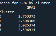
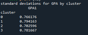

Students in cluster 2 had higher GPA values with an SD of 0.70 and cluster 1 had lower GPA values with an SD of 0.79
0 notes
Text
0 notes
Text
How do I learn Python?
Python is an excellent way to dive into the world of data science because it is very readable, versatile, and has huge ecosystems of libraries. Here is a roadmap to guide you:
1. Master the Basics:
The syntax of Python: This includes variables, data types, operators, control flow, and functions.
Practice regularly: To be a good coder, one needs to practice as one would while learning a language.
Web resources: Codecademy, LearnPython.org, and Google's Python tutorial provide interactive lessons.
2. Master Data Structures:
Know lists, tuples, dictionaries, sets: Start with the basics of how to manipulate data.
Know ops on, use cases for these data structures: How to create, modify, access data within
3. Important Libraries:
NumPy: Numerical computations, array operations
Pandas: Data manipulation, analysis, creation of DataFrames.
MatplotLib: To be used in the visualization of data through the plotting of different types of plots.
Seaborn: It is used in making beautiful statistical graphics.
4. Data Manipulation and Analysis
Loading and Understanding Datasets: From CSV to Excel, and more
Cleaning and Preprocessing Data: Missing values, outliers, inconsistencies
Implementing Exploratory Data Analysis: Summarization, looking for patterns, and visualizing insight
5. Machine Learning Using Scikit-learn
Core ML Concepts: Supervised, unsupervised learning, model evaluation
Implementing algorithms: Regression, classification, clustering, and more.
Tune models: Gain enhanced performance by tuning hyperparameters.
6. Deep Learning with TensorFlow/Keras
Learn neural networks, architecture, layers, and activation functions
Build and train models for deep learning on image recognition, natural language processing, etc.
7. Practice with Real-World Projects:
Kaggle competitions: Apply your skills to real-world problems
Personal projects: Explore your interests and create your datasets
Contributing to open-source projects: Engage with the community and learn from others.
Extras: Online communities like Stack Overflow, r/learnpython on Reddit, and a bunch of forums on data science can help a great deal as well.
Strong basics: Properly grasp the concepts of mathematics and statistics.
Experiment and iterate: Data science can be pretty iterative. It is totally all right to do things over again to see how things workout.
Remember: Learning data science is a journey. Start with the very basics; gradually build up level after level of skill, and most importantly, enjoy the process!
0 notes
Text
Learn The Art Of How To Tabulate Data in Python: Tips And Tricks
Summary: Master how to tabulate data in Python using essential libraries like Pandas and NumPy. This guide covers basic and advanced techniques, including handling missing data, multi-indexing, and creating pivot tables, enabling efficient Data Analysis and insightful decision-making.

Introduction
In Data Analysis, mastering how to tabulate data in Python is akin to wielding a powerful tool for extracting insights. This article offers a concise yet comprehensive overview of this essential skill. Analysts and Data Scientists can efficiently organise and structure raw information by tabulating data, paving the way for deeper analysis and visualisation.
Understanding the significance of tabulation lays the foundation for effective decision-making, enabling professionals to uncover patterns, trends, and correlations within datasets. Join us as we delve into the intricacies of data tabulation in Python, unlocking its potential for informed insights and impactful outcomes.
Getting Started with Data Tabulation Using Python
Tabulating data is a fundamental aspect of Data Analysis and is crucial in deriving insights and making informed decisions. With Python, a versatile and powerful programming language, you can efficiently tabulate data from various sources and formats.
Whether working with small-scale datasets or handling large volumes of information, Python offers robust tools and libraries to streamline the tabulation process. Understanding the basics is essential when tabulating data using Python. In this section, we'll delve into the foundational concepts of data tabulation and explore how Python facilitates this task.
Basic Data Structures for Tabulation
Before diving into data tabulation techniques, it's crucial to grasp the basic data structures commonly used in Python. These data structures are the building blocks for effectively organising and manipulating data. The primary data structures for tabulation include lists, dictionaries, and data frames.
Lists: Lists are versatile data structures in Python that allow you to store and manipulate sequences of elements. They can contain heterogeneous data types and are particularly useful for tabulating small-scale datasets.
Dictionaries: Dictionaries are collections of key-value pairs that enable efficient data storage and retrieval. They provide a convenient way to organise tabulated data, especially when dealing with structured information.
DataFrames: These are a central data structure in libraries like Pandas, offering a tabular data format similar to a spreadsheet or database table. DataFrames provide potent tools for tabulating and analysing data, making them a preferred choice for many Data Scientists and analysts.
Overview of Popular Python Libraries for Data Tabulation
Python boasts a rich ecosystem of libraries specifically designed for data manipulation and analysis. Two popular libraries for data tabulation are Pandas and NumPy.
Pandas: It is a versatile and user-friendly library that provides high-performance data structures and analysis tools. Pandas offers a DataFrame object and a wide range of functions for reading, writing, and manipulating tabulated data efficiently.
NumPy: It is a fundamental library for Python numerical computing. It provides support for large, multidimensional arrays and matrices. While not explicitly designed for tabulation, NumPy’s array-based operations are often used for data manipulation tasks with other libraries.
By familiarising yourself with these basic data structures and popular Python libraries, you'll be well-equipped to embark on your journey into data tabulation using Python.
Tabulating Data with Pandas
Pandas is a powerful Python library widely used for data manipulation and analysis. This section will delve into the fundamentals of tabulating data with Pandas, covering everything from installation to advanced operations.
Installing and Importing Pandas
Before tabulating data with Pandas, you must install the library on your system. Installation is typically straightforward using Python's package manager, pip. Open your command-line interface and execute the following command:
Once Pandas is installed, you can import it into your Python scripts or notebooks using the `import` statement:
Reading Data into Pandas DataFrame
Pandas provide various functions for reading data from different file formats such as CSV, Excel, SQL databases, etc. One of the most commonly used functions is `pd.read_csv()` for reading data from a CSV file into a Pandas DataFrame:
You can replace `'data.csv'` with the path to your CSV file. Pandas automatically detect the delimiter and other parameters to load the data correctly.
Basic DataFrame Operations for Tabulation
Once your data is loaded into a data frame, you can perform various operations to tabulate and manipulate it. Some basic operations include:
Selecting Data: Use square brackets `[]` or the `.loc[]` and `.iloc[]` accessors to select specific rows and columns.
Filtering Data: Apply conditional statements to filter rows based on specific criteria using boolean indexing.
Sorting Data: Use the `.sort_values()` method to sort the DataFrame by one or more columns.
Grouping and Aggregating Data with Pandas
Grouping and aggregating data are essential techniques for summarising and analysing datasets. Pandas provides the `.groupby()` method for grouping data based on one or more columns. After grouping, you can apply aggregation functions such as `sum()`, `mean()`, `count()`, etc., to calculate statistics for each group.
This code groups the DataFrame `df` by the 'category' column. It calculates the sum of the 'value' column for each group.
Mastering these basic operations with Pandas is crucial for efficient data tabulation and analysis in Python.
Advanced Techniques for Data Tabulation
Mastering data tabulation involves more than just basic operations. Advanced techniques can significantly enhance your data manipulation and analysis capabilities. This section explores how to handle missing data, perform multi-indexing, create pivot tables, and combine datasets for comprehensive tabulation.
Handling Missing Data in Tabulated Datasets
Missing data is a common issue in real-world datasets, and how you handle it can significantly affect your analysis. Python's Pandas library provides robust methods to manage missing data effectively.
First, identify missing data using the `isnull()` function, which helps locate NaNs in your DataFrame. You can then decide whether to remove or impute these values. Use `dropna()` to eliminate rows or columns with missing data. This method is straightforward but might lead to a significant data loss.
Alternatively, the `fillna()` method can fill missing values. This function allows you to replace NaNs with specific values, such as the mean and median, or a technique such as forward-fill or backward-fill. Choosing the right strategy depends on your dataset and analysis goals.
Performing Multi-Indexing and Hierarchical Tabulation
Multi-indexing, or hierarchical indexing, enables you to work with higher-dimensional data in a structured way. This technique is invaluable for managing complex datasets containing multiple information levels.
In Pandas, create a multi-index DataFrame by passing a list of arrays to the `set_index()` method. This approach allows you to perform operations across multiple levels. For instance, you can aggregate data at different levels using the `groupby()` function. Multi-indexing enhances your ability to navigate and analyse data hierarchically, making it easier to extract meaningful insights.
Pivot Tables for Advanced Data Analysis
Pivot tables are potent tools for summarising and reshaping data, making them ideal for advanced Data Analysis. You can create pivot tables in Python using Pandas `pivot_table()` function.
A pivot table lets you group data by one or more keys while applying an aggregate function, such as sum, mean, or count. This functionality simplifies data comparison and trend identification across different dimensions. By specifying parameters like `index`, `columns`, and `values`, you can customise the table to suit your analysis needs.
Combining and Merging Datasets for Comprehensive Tabulation
Combining and merging datasets is essential when dealing with fragmented data sources. Pandas provides several functions to facilitate this process, including `concat()`, `merge()`, and `join()`.
Use `concat()` to append or stack DataFrames vertically or horizontally. This function helps add new data to an existing dataset. Like SQL joins, the `merge()` function combines datasets based on standard columns or indices. This method is perfect for integrating related data from different sources. The `join()` function offers a more straightforward way to merge datasets on their indices, simplifying the combination process.
These advanced techniques can enhance your data tabulation skills, leading to more efficient and insightful Data Analysis.
Tips and Tricks for Efficient Data Tabulation
Efficient data tabulation in Python saves time and enhances the quality of your Data Analysis. Here, we'll delve into some essential tips and tricks to optimise your data tabulation process.
Utilising Vectorised Operations for Faster Tabulation
Vectorised operations in Python, particularly with libraries like Pandas and NumPy, can significantly speed up data tabulation. These operations allow you to perform computations on entire arrays or DataFrames without explicit loops.
You can leverage the underlying C and Fortran code in these libraries using vectorised operations, much faster than Python's native loops. For instance, consider adding two columns in a DataFrame. Instead of using a loop to iterate through each row, you can simply use:
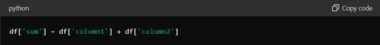
This one-liner makes your code more concise and drastically reduces execution time. Embrace vectorisation whenever possible to maximise efficiency.
Optimising Memory Usage When Working with Large Datasets
Large datasets can quickly consume your system's memory, leading to slower performance or crashes. Optimising memory usage is crucial for efficient data tabulation.
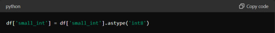
One effective approach is to use appropriate data types for your columns. For instance, if you have a column of integers that only contains values from 0 to 255, using the `int8` data type instead of the default `int64` can save substantial memory. Here's how you can optimise a DataFrame:
Additionally, consider using chunking techniques when reading large files. Instead of loading the entire dataset at once, process it in smaller chunks:
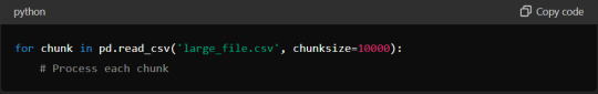
This method ensures you never exceed your memory capacity, maintaining efficient data processing.
Customising Tabulated Output for Readability and Presentation
Presenting your tabulated data is as important as the analysis itself. Customising the output can enhance readability and make your insights more accessible.
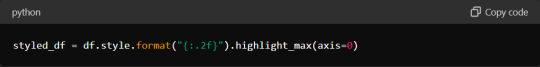
Start by formatting your DataFrame using Pandas' built-in styling functions. You can highlight important data points, format numbers, and even create colour gradients. For example:
Additionally, when exporting data to formats like CSV or Excel, ensure that headers and index columns are appropriately labelled. Use the `to_csv` and `to_excel` methods with options for customisation:
These small adjustments can significantly improve the presentation quality of your tabulated data.
Leveraging Built-in Functions and Methods for Streamlined Tabulation
Python libraries offer many built-in functions and methods that simplify and expedite the tabulation process. Pandas, in particular, provide powerful tools for data manipulation.
For instance, the `groupby` method allows you to group data by specific columns and perform aggregate functions such as sum, mean, or count:
Similarly, the `pivot_table` method lets you create pivot tables, which are invaluable for summarising and analysing large datasets.
Mastering these built-in functions can streamline your data tabulation workflow, making it faster and more effective.
Incorporating these tips and tricks into your data tabulation process will enhance efficiency, optimise resource usage, and improve the clarity of your presented data, ultimately leading to more insightful and actionable analysis.
Read More:
Data Abstraction and Encapsulation in Python Explained.
Anaconda vs Python: Unveiling the differences.
Frequently Asked Questions
What Are The Basic Data Structures For Tabulating Data In Python?
Lists, dictionaries, and DataFrames are the primary data structures for tabulating data in Python. Lists store sequences of elements, dictionaries manage key-value pairs, and DataFrames, available in the Pandas library, offer a tabular format for efficient Data Analysis.
How Do You Handle Missing Data In Tabulated Datasets Using Python?
To manage missing data in Python, use Pandas' `isnull()` to identify NaNs. Then, use `dropna()` to remove them or `fillna()` to replace them with appropriate values like the mean or median, ensuring data integrity.
What Are Some Advanced Techniques For Data Tabulation In Python?
Advanced tabulation techniques in Python include handling missing data, performing multi-indexing for hierarchical data, creating pivot tables for summarisation, and combining datasets using functions like `concat()`, `merge()`, and `join()` for comprehensive Data Analysis.
Conclusion
Mastering how to tabulate data in Python is essential for Data Analysts and scientists. Professionals can efficiently organise, manipulate, and analyse data by understanding and utilising Python's powerful libraries, such as Pandas and NumPy.
Techniques like handling missing data, multi-indexing, and creating pivot tables enhance the depth of analysis. Efficient data tabulation saves time and optimises memory usage, leading to more insightful and actionable outcomes. Embracing these skills will significantly improve data-driven decision-making processes.
0 notes
Text
K-means clusthering
#importamos las librerías necesarias
from pandas import Series,DataFrame
import pandas as pd
import numpy as np
import matplotlib.pylab as plt
from sklearn.model_selection
import train_test_splitfrom sklearn
import preprocessing
from sklearn.cluster import KMeans
"""Data Management"""
data =pd.read_csv("/content/drive/MyDrive/tree_addhealth.csv" )
#upper-case all DataFrame column names
data.columns = map(str.upper, data.columns)
# Data Managementdata_clean = data.dropna()
# subset clustering variablescluster=data_clean[['ALCEVR1','MAREVER1','ALCPROBS1','DEVIANT1','VIOL1','DEP1','ESTEEM1','SCHCONN1','PARACTV', 'PARPRES','FAMCONCT']]
cluster.describe()
# standardize clustering variables to have mean=0 and sd=1
clustervar=cluster.copy()
clustervar['ALCEVR1']=preprocessing.scale(clustervar['ALCEVR1'].astype('float64'))
clustervar['ALCPROBS1']=preprocessing.scale(clustervar['ALCPROBS1'].astype('float64'))
clustervar['MAREVER1']=preprocessing.scale(clustervar['MAREVER1'].astype('float64'))
clustervar['DEP1']=preprocessing.scale(clustervar['DEP1'].astype('float64'))
clustervar['ESTEEM1']=preprocessing.scale(clustervar['ESTEEM1'].astype('float64'))
clustervar['VIOL1']=preprocessing.scale(clustervar['VIOL1'].astype('float64'))
clustervar['DEVIANT1']=preprocessing.scale(clustervar['DEVIANT1'].astype('float64'))
clustervar['FAMCONCT']=preprocessing.scale(clustervar['FAMCONCT'].astype('float64'))
clustervar['SCHCONN1']=preprocessing.scale(clustervar['SCHCONN1'].astype('float64'))
clustervar['PARACTV']=preprocessing.scale(clustervar['PARACTV'].astype('float64'))
clustervar['PARPRES']=preprocessing.scale(clustervar['PARPRES'].astype('float64'))
# split data into train and test sets
clus_train, clus_test = train_test_split(clustervar, test_size=.3, random_state=123)
# k-means cluster analysis for 1-9 clusters
from scipy.spatial.distance import cdist
clusters=range(1,10)
meandist=[]
for k in clusters: model=KMeans(n_clusters=k) model.fit(clus_train) clusassign=model.predict(clus_train) meandist.append(sum(np.min(cdist(clus_train, model.cluster_centers_, 'euclidean'), axis=1))
/ clus_train.shape[0])
"""Plot average distance from observations from the cluster centroidto use the Elbow Method to identify number of clusters to choose"""
plt.plot(clusters,meandist)
plt.xlabel('Number of clusters')
plt.ylabel('Average distance')
plt.title('Selecting k with the Elbow Method')
# Interpret 2 cluster solution
model2=KMeans(n_clusters=2)model2.fit(clus_train)
clusassign=model2.predict(clus_train)
# plot clusters
from sklearn.decomposition import PCA
pca_2 = PCA(2)
plot_columns = pca_2.fit_transform(clus_train)
plt.scatter(x=plot_columns[:,0],y=plot_columns[:,1],c=model2.labels_,)
plt.xlabel('Canonical variable 1')
plt.ylabel('Canonical variable 2')
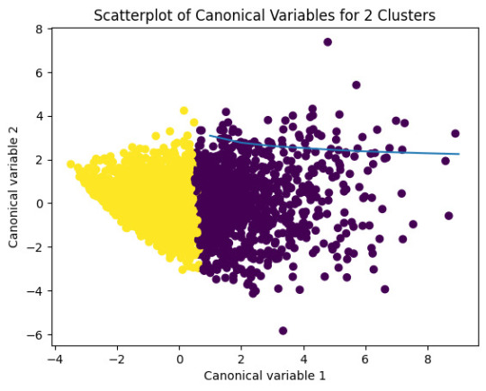
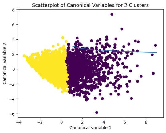
plt.title('Scatterplot of Canonical Variables for 2 Clusters')
plt.show()
"""BEGIN multiple steps to merge cluster assignment with clustering variables to examinecluster variable means by cluster"""
# create a unique identifier variable from the index for the
# cluster training data to merge with the cluster assignment variable
clus_train.reset_index(level=0, inplace=True)
# create a list that has the new index variable
cluslist=list(clus_train['index'])
# create a list of cluster assignments
labels=list(model2.labels_)
# combine index variable list with cluster assignment list into a dictionary
newlist=dict(zip(cluslist, labels))newlist
# convert newlist dictionary to a dataframenew
clus=DataFrame.from_dict(newlist, orient='index')newclus
# rename the cluster assignment columnnew
clus.columns = ['cluster']
# now do the same for the cluster assignment variable
# create a unique identifier variable from the index for the
# cluster assignment dataframe
# to merge with cluster training datanew
clus.reset_index(level=0, inplace=True)
# merge the cluster assignment dataframe with the cluster training variable dataframe
# by the index variablemerged_train=pd.merge(clus_train, newclus, on='index')
merged_train.head(n=100)
# cluster frequenciesmerged_train.cluster.value_counts()
"""END multiple steps to merge cluster assignment with clustering variables to examinecluster variable means by cluster"""
# FINALLY calculate clustering variable means by
clusterclustergrp = merged_train.groupby('cluster').mean()print ("Clustering variable means by cluster")
print(clustergrp)
# validate clusters in training data by examining cluster differences in GPA using ANOVA
# first have to merge GPA with clustering variables and cluster assignment data
gpa_data=data_clean['GPA1']
# split GPA data into train and test sets
gpa_train, gpa_test = train_test_split(gpa_data, test_size=.3, random_state=123)
gpa_train1=pd.DataFrame(gpa_train)
gpa_train1.reset_index(level=0, inplace=True)
merged_train_all=pd.merge(gpa_train1, merged_train, on='index')
sub1 = merged_train_all[['GPA1', 'cluster']].dropna()
import statsmodels.formula.api as smf
import statsmodels.stats.multicomp as multi
gpamod = smf.ols(formula='GPA1 ~ C(cluster)', data=sub1).fit()
print (gpamod.summary())
print ('means for GPA by cluster')
m1= sub1.groupby('cluster').mean()
print (m1)
print ('standard deviations for GPA by cluster')
m2= sub1.groupby('cluster').std()print (m2)
mc1 = multi.MultiComparison(sub1['GPA1'], sub1['cluster'])
res1 = mc1.tukeyhsd()
print(res1.summary())
爆發
0 則迴響
0 notes
Text
K-means clusthering
#importamos las librerías necesarias
from pandas import Series,DataFrame
import pandas as pd
import numpy as np
import matplotlib.pylab as plt
from sklearn.model_selection
import train_test_splitfrom sklearn
import preprocessing
from sklearn.cluster import KMeans
"""Data Management"""
data =pd.read_csv("/content/drive/MyDrive/tree_addhealth.csv" )
#upper-case all DataFrame column names
data.columns = map(str.upper, data.columns)
# Data Managementdata_clean = data.dropna()
# subset clustering variablescluster=data_clean[['ALCEVR1','MAREVER1','ALCPROBS1','DEVIANT1','VIOL1','DEP1','ESTEEM1','SCHCONN1','PARACTV', 'PARPRES','FAMCONCT']]
cluster.describe()
# standardize clustering variables to have mean=0 and sd=1
clustervar=cluster.copy()
clustervar['ALCEVR1']=preprocessing.scale(clustervar['ALCEVR1'].astype('float64'))
clustervar['ALCPROBS1']=preprocessing.scale(clustervar['ALCPROBS1'].astype('float64'))
clustervar['MAREVER1']=preprocessing.scale(clustervar['MAREVER1'].astype('float64'))
clustervar['DEP1']=preprocessing.scale(clustervar['DEP1'].astype('float64'))
clustervar['ESTEEM1']=preprocessing.scale(clustervar['ESTEEM1'].astype('float64'))
clustervar['VIOL1']=preprocessing.scale(clustervar['VIOL1'].astype('float64'))
clustervar['DEVIANT1']=preprocessing.scale(clustervar['DEVIANT1'].astype('float64'))
clustervar['FAMCONCT']=preprocessing.scale(clustervar['FAMCONCT'].astype('float64'))
clustervar['SCHCONN1']=preprocessing.scale(clustervar['SCHCONN1'].astype('float64'))
clustervar['PARACTV']=preprocessing.scale(clustervar['PARACTV'].astype('float64'))
clustervar['PARPRES']=preprocessing.scale(clustervar['PARPRES'].astype('float64'))
# split data into train and test sets
clus_train, clus_test = train_test_split(clustervar, test_size=.3, random_state=123)
# k-means cluster analysis for 1-9 clusters
from scipy.spatial.distance import cdist
clusters=range(1,10)
meandist=[]
for k in clusters: model=KMeans(n_clusters=k) model.fit(clus_train) clusassign=model.predict(clus_train) meandist.append(sum(np.min(cdist(clus_train, model.cluster_centers_, 'euclidean'), axis=1))
/ clus_train.shape[0])
"""Plot average distance from observations from the cluster centroidto use the Elbow Method to identify number of clusters to choose"""
plt.plot(clusters,meandist)
plt.xlabel('Number of clusters')
plt.ylabel('Average distance')
plt.title('Selecting k with the Elbow Method')
# Interpret 2 cluster solution
model2=KMeans(n_clusters=2)model2.fit(clus_train)
clusassign=model2.predict(clus_train)
# plot clusters
from sklearn.decomposition import PCA
pca_2 = PCA(2)
plot_columns = pca_2.fit_transform(clus_train)
plt.scatter(x=plot_columns[:,0],y=plot_columns[:,1],c=model2.labels_,)
plt.xlabel('Canonical variable 1')
plt.ylabel('Canonical variable 2')
plt.title('Scatterplot of Canonical Variables for 2 Clusters')
plt.show()
"""BEGIN multiple steps to merge cluster assignment with clustering variables to examinecluster variable means by cluster"""
# create a unique identifier variable from the index for the
# cluster training data to merge with the cluster assignment variable
clus_train.reset_index(level=0, inplace=True)
# create a list that has the new index variable
cluslist=list(clus_train['index'])
# create a list of cluster assignments
labels=list(model2.labels_)
# combine index variable list with cluster assignment list into a dictionary
newlist=dict(zip(cluslist, labels))newlist
# convert newlist dictionary to a dataframenew
clus=DataFrame.from_dict(newlist, orient='index')newclus
# rename the cluster assignment columnnew
clus.columns = ['cluster']
# now do the same for the cluster assignment variable
# create a unique identifier variable from the index for the
# cluster assignment dataframe
# to merge with cluster training datanew
clus.reset_index(level=0, inplace=True)
# merge the cluster assignment dataframe with the cluster training variable dataframe
# by the index variablemerged_train=pd.merge(clus_train, newclus, on='index')
merged_train.head(n=100)
# cluster frequenciesmerged_train.cluster.value_counts()
"""END multiple steps to merge cluster assignment with clustering variables to examinecluster variable means by cluster"""
# FINALLY calculate clustering variable means by
clusterclustergrp = merged_train.groupby('cluster').mean()print ("Clustering variable means by cluster")
print(clustergrp)
# validate clusters in training data by examining cluster differences in GPA using ANOVA
# first have to merge GPA with clustering variables and cluster assignment data
gpa_data=data_clean['GPA1']
# split GPA data into train and test sets
gpa_train, gpa_test = train_test_split(gpa_data, test_size=.3, random_state=123)
gpa_train1=pd.DataFrame(gpa_train)
gpa_train1.reset_index(level=0, inplace=True)
merged_train_all=pd.merge(gpa_train1, merged_train, on='index')
sub1 = merged_train_all[['GPA1', 'cluster']].dropna()
import statsmodels.formula.api as smf
import statsmodels.stats.multicomp as multi
gpamod = smf.ols(formula='GPA1 ~ C(cluster)', data=sub1).fit()
print (gpamod.summary())
print ('means for GPA by cluster')
m1= sub1.groupby('cluster').mean()
print (m1)
print ('standard deviations for GPA by cluster')
m2= sub1.groupby('cluster').std()print (m2)
mc1 = multi.MultiComparison(sub1['GPA1'], sub1['cluster'])
res1 = mc1.tukeyhsd()
print(res1.summary())
0 notes
Text
Python Data Science Essentials: Beginner's Guide to Analyzing Data
Introduction:
In today's data-driven world, the ability to analyze and interpret data is becoming increasingly valuable. Python, with its simplicity and versatility, has emerged as a powerful tool for data science. Whether you're a beginner or an experienced programmer, Python offers a wide range of libraries and tools tailored for data analysis. In this beginner's guide, we'll explore the essentials of using Python for data science, breaking down complex concepts into easy-to-understand language.
Why Python for Data Science?
Python has gained immense popularity in the field of data science due to several reasons. Its simple syntax makes it easy to learn for beginners, while its robust libraries offer advanced functionalities for data analysis. Additionally, Python enjoys strong community support, with a vast ecosystem of resources, tutorials, and forums available for assistance.
Setting Up Your Python Environment
Before diving into data analysis, you'll need to set up your Python environment. Start by installing Python from the official website (python.org) or using a distribution like Anaconda, which comes bundled with popular data science libraries such as NumPy, pandas, and Matplotlib. Once installed, you can use an integrated development environment (IDE) like Jupyter Notebook or Visual Studio Code for coding.
Understanding Data Structures in Python
Python offers various data structures that are essential for data manipulation and analysis. These include lists, tuples, dictionaries, and sets. Understanding how these data structures work will greatly enhance your ability to handle and process data effectively.
Introduction to NumPy and Pandas
NumPy and Pandas are two fundamental libraries for data manipulation in Python. NumPy provides support for large, multi-dimensional arrays and matrices, along with a collection of mathematical functions to operate on these arrays. Pandas, on the other hand, offers data structures like DataFrame and Series, which are ideal for handling structured data.
Data Visualization with Matplotlib and Seaborn
Visualizing data is crucial for gaining insights and communicating findings effectively. Matplotlib and Seaborn are popular Python libraries for creating static, interactive, and publication-quality visualizations. From simple line plots to complex heatmaps, these libraries offer a wide range of plotting functionalities.
Exploratory Data Analysis (EDA)
Exploratory Data Analysis (EDA) is the process of analyzing data sets to summarize their main characteristics, often employing visual methods. Python's libraries, such as Pandas and Matplotlib, facilitate EDA by providing tools for data manipulation and visualization. Through EDA, you can uncover patterns, detect anomalies, and formulate hypotheses about the underlying data.
Introduction to Machine Learning with Scikit-Learn
Machine learning is a subset of artificial intelligence that enables systems to learn from data without being explicitly programmed. Scikit-Learn is a powerful machine learning library in Python, offering a wide range of algorithms for classification, regression, clustering, and more. By leveraging Scikit-Learn, you can build predictive models and make data-driven decisions.
Data Cleaning and Preprocessing
Before applying machine learning algorithms to your data, it's essential to clean and preprocess it to ensure accuracy and reliability. Python provides tools for handling missing values, removing outliers, encoding categorical variables, and scaling features. By preprocessing your data effectively, you can improve the performance of your machine learning models.
Conclusion: Embracing Python for Data Science
In conclusion, Python serves as a versatile and accessible platform for data science, offering a rich ecosystem of libraries and tools for every stage of the data analysis pipeline. Whether you're exploring data, building predictive models, or visualizing insights, Python provides the necessary resources to unlock the potential of your data. By mastering the essentials outlined in this guide, you'll be well-equipped to embark on your journey into the fascinating world of data science.
In this article, we've covered the fundamental aspects of using Python for data science, from setting up your environment to performing exploratory data analysis and building machine learning models. With its user-friendly syntax and powerful libraries, Python empowers beginners and professionals alike to extract valuable insights from data and drive informed decision-making. So, whether you're a curious enthusiast or a seasoned data scientist, Python is your gateway to the exciting field of data science.
0 notes
Text
KMeans Clustering Assignment
Import the modules
from pandas import Series, DataFrame import pandas as pd import numpy as np import matplotlib.pylab as plt from sklearn.model_selection import train_test_split from sklearn import preprocessing from sklearn.cluster import KMeans
Load the dataset
data = pd.read_csv("C:\Users\guy3404\OneDrive - MDLZ\Documents\Cross Functional Learning\AI COP\Coursera\machine_learning_data_analysis\Datasets\tree_addhealth.csv")
data.head()
upper-case all DataFrame column names
data.columns = map(str.upper, data.columns)
Data Management
data_clean = data.dropna() data_clean.head()
subset clustering variables
cluster=data_clean[['ALCEVR1','MAREVER1','ALCPROBS1','DEVIANT1','VIOL1', 'DEP1','ESTEEM1','SCHCONN1','PARACTV', 'PARPRES','FAMCONCT']] cluster.describe()

standardize clustering variables to have mean=0 and sd=1
clustervar=cluster.copy() clustervar['ALCEVR1']=preprocessing.scale(clustervar['ALCEVR1'].astype('float64')) clustervar['ALCPROBS1']=preprocessing.scale(clustervar['ALCPROBS1'].astype('float64')) clustervar['MAREVER1']=preprocessing.scale(clustervar['MAREVER1'].astype('float64')) clustervar['DEP1']=preprocessing.scale(clustervar['DEP1'].astype('float64')) clustervar['ESTEEM1']=preprocessing.scale(clustervar['ESTEEM1'].astype('float64')) clustervar['VIOL1']=preprocessing.scale(clustervar['VIOL1'].astype('float64')) clustervar['DEVIANT1']=preprocessing.scale(clustervar['DEVIANT1'].astype('float64')) clustervar['FAMCONCT']=preprocessing.scale(clustervar['FAMCONCT'].astype('float64')) clustervar['SCHCONN1']=preprocessing.scale(clustervar['SCHCONN1'].astype('float64')) clustervar['PARACTV']=preprocessing.scale(clustervar['PARACTV'].astype('float64')) clustervar['PARPRES']=preprocessing.scale(clustervar['PARPRES'].astype('float64'))
split data into train and test sets
clus_train, clus_test = train_test_split(clustervar, test_size=.3, random_state=123)
k-means cluster analysis for 1-9 clusters
from scipy.spatial.distance import cdist clusters=range(1,10) meandist=[]
for k in clusters: model=KMeans(n_clusters=k) model.fit(clus_train) clusassign=model.predict(clus_train) meandist.append(sum(np.min(cdist(clus_train, model.cluster_centers_, 'euclidean'), axis=1)) / clus_train.shape[0])
""" Plot average distance from observations from the cluster centroid to use the Elbow Method to identify number of clusters to choose """ plt.plot(clusters, meandist) plt.xlabel('Number of clusters') plt.ylabel('Average distance') plt.title('Selecting k with the Elbow Method')
Interpret 3 cluster solution
model3=KMeans(n_clusters=3) model3.fit(clus_train) clusassign=model3.predict(clus_train)
plot clusters
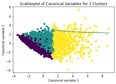
from sklearn.decomposition import PCA pca_2 = PCA(2) plot_columns = pca_2.fit_transform(clus_train) plt.scatter(x=plot_columns[:,0], y=plot_columns[:,1], c=model3.labels_,) plt.xlabel('Canonical variable 1') plt.ylabel('Canonical variable 2') plt.title('Scatterplot of Canonical Variables for 3 Clusters') plt.show()
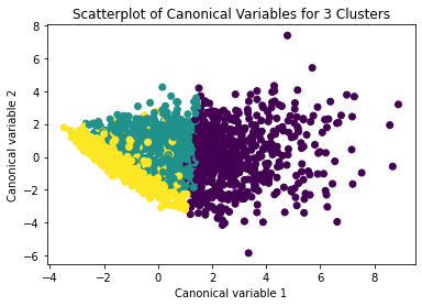
The datapoints of the 2 clusters in the left are less spread out but have more overlaps. The cluster to the right is more distinct but has more spread in the data points
""" BEGIN multiple steps to merge cluster assignment with clustering variables to examine cluster variable means by cluster """
create a unique identifier variable from the index for the
cluster training data to merge with the cluster assignment variable
clus_train.reset_index(level=0, inplace=True)
create a list that has the new index variable
cluslist=list(clus_train['index'])
create a list of cluster assignments
labels=list(model3.labels_)
combine index variable list with cluster assignment list into a dictionary
newlist=dict(zip(cluslist, labels)) newlist
convert newlist dictionary to a dataframe
newclus=DataFrame.from_dict(newlist, orient='index') newclus
rename the cluster assignment column
newclus.columns = ['cluster']
now do the same for the cluster assignment variable
create a unique identifier variable from the index for the
cluster assignment dataframe
to merge with cluster training data
newclus.reset_index(level=0, inplace=True)
merge the cluster assignment dataframe with the cluster training variable dataframe
by the index variable
merged_train=pd.merge(clus_train, newclus, on='index') merged_train.head(n=100)
cluster frequencies
merged_train.cluster.value_counts()
""" END multiple steps to merge cluster assignment with clustering variables to examine cluster variable means by cluster """
FINALLY calculate clustering variable means by cluster
clustergrp = merged_train.groupby('cluster').mean() print ("Clustering variable means by cluster") print(clustergrp)
validate clusters in training data by examining cluster differences in GPA using ANOVA
first have to merge GPA with clustering variables and cluster assignment data
gpa_data=data_clean['GPA1']
split GPA data into train and test sets
gpa_train, gpa_test = train_test_split(gpa_data, test_size=.3, random_state=123) gpa_train1=pd.DataFrame(gpa_train) gpa_train1.reset_index(level=0, inplace=True) merged_train_all=pd.merge(gpa_train1, merged_train, on='index') sub1 = merged_train_all[['GPA1', 'cluster']].dropna()
Print statistical summary by cluster
import statsmodels.formula.api as smf import statsmodels.stats.multicomp as multi
gpamod = smf.ols(formula='GPA1 ~ C(cluster)', data=sub1).fit() print (gpamod.summary())
print ('means for GPA by cluster') m1= sub1.groupby('cluster').mean() print (m1)
print ('standard deviations for GPA by cluster') m2= sub1.groupby('cluster').std() print (m2)
Interpretation
The clustering average summary shows Cluster 0 has higher alcohol and marijuana problems, shows higher deviant and violent behavior, suffers from depression, has low self esteem,school connectedness, paraental and family connectedness. On the contrary, Cluster 2 shows the lowest alcohol and marijuana problems, lowest deviant & violent behavior,depression, and higher self esteem,school connectedness, paraental and family connectedness. Further, when validated against GPA score, we observe Cluster 0 shows the lowest average GPA and CLuster 2 has the highest average GPA which aligns with the summary statistics interpretation.
1 note
·
View note
Text
Mastering Python for Data Science: A Step-by-Step Guide

Data science is transforming industries around the world, from healthcare to finance, by leveraging the power of data to generate actionable insights. Python, a powerful and multipurpose programming language, is used by data scientists to clean, analyze, and visualize data. It is also used to build machine learning models and algorithms. Python is a popular choice for data science because it is easy to learn, has a large community of users, and is well supported by libraries and tools.
In this article, we will walk you through the journey of mastering Python for data science, step by step. We will also explore various aspects of data science using Python. By the end, you’ll not only have a solid foundation in Python but also a clear path forward in your data science career.
Learning Python for Data Science:
Before we dive into the details, let’s address the elephant in the room: why Python? Python has become the go-to language for data science for several reasons.
Readability and Simplicity: Python’s clean and readable syntax makes it easy for data scientists to express complex ideas with less code. This means faster development and easier collaboration.
Extensive Libraries: Python boasts a rich ecosystem of libraries, including NumPy, Pandas, Matplotlib, and Scikit-Learn, which provide powerful tools for data manipulation, analysis, and visualization.
Community Support: Python has a vibrant and active community. If you encounter a problem or need assistance, chances are someone has already faced a similar issue and found a solution.
Multipurpose: Python is not limited to data science. It can be used for web development, automation, machine learning, and more. Learning Python opens up a world of possibilities beyond data science.
The Python Basics
The first step is to learn the fundamentals of Python. Even if you’re an absolute beginner, Python’s ease of use makes it accessible to anyone. Begin with fundamental concepts such as variables, data types, and basic operations. Here are a few key points:
Variables: In Python, you don’t need to declare the data type explicitly. Just assign a value, and Python figures out the rest.
Data Types: Python supports various data types, including integers, floats, strings, lists, and dictionaries. Understanding when to use each is crucial.
Basic Operations: Learn how to perform arithmetic operations, concatenate strings, and manipulate data with built-in functions.
Control Structures: Master if-else statements, loops, and other control structures to control the flow of your programs.
Pro Tip: To solidify your understanding, practice coding regularly. Sites like LeetCode and HackerRank offer plenty of Python exercises to sharpen your skills.
Data Manipulation with NumPy and Pandas
Once you’ve got a handle on Python basics, it’s time to dive into data manipulation, and that’s where NumPy and Pandas come in.
NumPy: NumPy is the foundation for scientific computing in Python. It provides support for arrays and matrices, along with mathematical functions to operate on them efficiently. This makes it a powerful tool for data analysis, machine learning, and other scientific applications.
Pandas: Pandas, a Python library, simplifies structured data handling. You can easily create, clean, and analyze datasets using its versatile data structures, primarily DataFrames and Series. Mastering Pandas is essential for effective data manipulation and analysis tasks.
Data Cleaning: Data cleaning is an essential step in data analysis. It involves various techniques to handle missing data, outliers, and duplicates, ensuring that your datasets are accurate and ready for analysis. Understanding these techniques is crucial for reliable data-driven insights.
Data Visualization with Matplotlib
Data visualization is a vital aspect of data science. Matplotlib is a versatile library for creating stunning visualizations.
Plotting Basics: Learn how to create various types of plots, including line plots, bar charts, histograms, and scatter plots.
A line plot is a type of graph that shows the relationship between two variables.
A bar chart is a type of graph that shows the frequency of data points.
A histogram is a type of graph that shows the distribution of data.
A scatter plot is a type of graph that shows the relationship between two variables.
These are just a few of the many types of plots that can be created. The type of plot that is best for a particular data set will depend on the type of data and the question that is being asked.
Customization: Explore Matplotlib’s customization options to make your visualizations informative and aesthetically pleasing.
Seaborn: Additionally, consider learning Seaborn. Seaborn is a higher-level interface for Matplotlib that simplifies complex data visualizations. It provides a collection of high-level functions for drawing attractive and informative statistical graphics.
Machine Learning with Scikit-Learn
Now that you have a solid foundation in Python and data manipulation, it’s time to step into the world of machine learning.
Introduction to Machine Learning: Understand the basic concepts of supervised and unsupervised learning, as well as common machine learning algorithms.
Scikit-Learn: Explore the Scikit-Learn library, which provides a straightforward interface for implementing machine learning models. It provides an intuitive interface for deploying a variety of machine learning models. Scikit-Learn equips data professionals with essential model building and analysis capabilities.
Hands-on Projects: Apply your newfound knowledge by working on real-world projects, such as building predictive models or clustering datasets.
Data Analysis with Python
Data analysis is a crucial component of the data science process. In this step, you’ll learn how to dig deeper into datasets, extract meaningful insights, and make data-driven decisions.
Exploratory Data Analysis (EDA): Discover how to perform EDA to gain a deeper understanding of your data. Explore summary statistics, data distributions, and visualize trends and patterns.
Hypothesis Testing: Learn the fundamentals of hypothesis testing to make informed decisions based on statistical significance.
Data Visualization for Analysis: Data visualization is a powerful tool that can help you communicate your findings effectively. By creating insightful visualizations, you can help your audience understand complex data in a way that is easy to see and understand. Data visualization can help you spot trends and patterns in your data. It’s a great way to improve your data analysis skills.
Pandas for Advanced Data Manipulation: Dive deeper into Pandas to perform advanced data transformations, groupings, and aggregations.
Time Series Analysis: If applicable to your domain, explore time series data analysis techniques for forecasting and trend analysis.
Real-World Data Science Projects
To truly master Python for data science, it’s essential to apply your skills to real-world projects. Joining a data science community or collaborating on open-source projects can provide invaluable experience.
Open-Source Contributions: Consider contributing to open-source data science projects. It’s an excellent way to collaborate with experienced data scientists and showcase your skills.
Personal Projects: Create your data science portfolio by working on personal projects that interest you. This can be anything from analyzing a favorite dataset to solving a specific problem.
Take Your Learning to the Next Level with Datavalley’s Data Science Course
To accelerate your journey in mastering Python for data science, consider enrolling in Datavalley’s Data Science Course. Our comprehensive program covers everything discussed in this guide and more, with expert instructors and hands-on projects to reinforce your learning.
In-Depth Curriculum: Our course offers an in-depth curriculum that covers Python for data science, artificial intelligence, statistics and linear algebra, machine learning, cloud computing, and real-world projects.
Expert Guidance: Learn from experienced data scientists who provide personalized guidance and support throughout your learning journey.
Hands-On Projects: Apply your knowledge to real-world projects, building a strong portfolio that impresses potential employers.
Project-Ready, Not Just Job-Ready: Upon completion of our program, you will be prepared to begin working immediately and confidently execute projects.
Community Engagement: Join a vibrant community of data science enthusiasts, collaborate on projects, and network with like-minded individuals.
On-call Project Assistance After Landing Your Dream Job: Our experts can provide you with up to 3 months of on-call project assistance to help you succeed in your new role.
Make use of this opportunity to take your data science skills to the next level. Enroll in Datavalley’s Advanced Data Science Master Program today and open the door to a world of data-driven possibilities!
Conclusion
Mastering Python for data science is an essential step towards a satisfying career in this field. With a strong foundation in Python, data manipulation, visualization, machine learning, data analysis, and practical experience, you’ll be well-prepared to tackle real-world data challenges.
Remember, learning is a continuous journey. Stay curious, explore new datasets, and keep up with the latest developments in data science. Whether you’re a beginner or an experienced professional, the world of data science offers endless opportunities for growth and innovation. Start your journey today!
#datavalley#data science#data science certification#data science course#data science training#data scientist#datavalleyai
0 notes
Text
rom pandas import Series, DataFrame import pandas as pd import numpy as np import matplotlib.pylab as plt from sklearn.model_selection import train_test_split from sklearn import preprocessing from sklearn.cluster import KMeans
""" Data Management """ data = pd.read_csv("tree_addhealth")
upper-case all DataFrame column names
data.columns = map(str.upper, data.columns)
Data Management
data_clean = data.dropna()
subset clustering variables
cluster=data_clean[['ALCEVR1','MAREVER1','ALCPROBS1','DEVIANT1','VIOL1', 'DEP1','ESTEEM1','SCHCONN1','PARACTV', 'PARPRES','FAMCONCT']] cluster.describe()
standardize clustering variables to have mean=0 and sd=1
clustervar=cluster.copy() clustervar['ALCEVR1']=preprocessing.scale(clustervar['ALCEVR1'].astype('float64')) clustervar['ALCPROBS1']=preprocessing.scale(clustervar['ALCPROBS1'].astype('float64')) clustervar['MAREVER1']=preprocessing.scale(clustervar['MAREVER1'].astype('float64')) clustervar['DEP1']=preprocessing.scale(clustervar['DEP1'].astype('float64')) clustervar['ESTEEM1']=preprocessing.scale(clustervar['ESTEEM1'].astype('float64')) clustervar['VIOL1']=preprocessing.scale(clustervar['VIOL1'].astype('float64')) clustervar['DEVIANT1']=preprocessing.scale(clustervar['DEVIANT1'].astype('float64')) clustervar['FAMCONCT']=preprocessing.scale(clustervar['FAMCONCT'].astype('float64')) clustervar['SCHCONN1']=preprocessing.scale(clustervar['SCHCONN1'].astype('float64')) clustervar['PARACTV']=preprocessing.scale(clustervar['PARACTV'].astype('float64')) clustervar['PARPRES']=preprocessing.scale(clustervar['PARPRES'].astype('float64'))
split data into train and test sets
clus_train, clus_test = train_test_split(clustervar, test_size=.3, random_state=123)
k-means cluster analysis for 1-9 clusters
from scipy.spatial.distance import cdist clusters=range(1,10) meandist=[]
for k in clusters: model=KMeans(n_clusters=k) model.fit(clus_train) clusassign=model.predict(clus_train) meandist.append(sum(np.min(cdist(clus_train, model.cluster_centers_, 'euclidean'), axis=1)) / clus_train.shape[0])
""" Plot average distance from observations from the cluster centroid to use the Elbow Method to identify number of clusters to choose """
plt.plot(clusters, meandist) plt.xlabel('Number of clusters') plt.ylabel('Average distance') plt.title('Selecting k with the Elbow Method')
Interpret 3 cluster solution
model3=KMeans(n_clusters=3) model3.fit(clus_train) clusassign=model3.predict(clus_train)
plot clusters
from sklearn.decomposition import PCA pca_2 = PCA(2) plot_columns = pca_2.fit_transform(clus_train) plt.scatter(x=plot_columns[:,0], y=plot_columns[:,1], c=model3.labels_,) plt.xlabel('Canonical variable 1') plt.ylabel('Canonical variable 2') plt.title('Scatterplot of Canonical Variables for 3 Clusters') plt.show()
""" BEGIN multiple steps to merge cluster assignment with clustering variables to examine cluster variable means by cluster """
create a unique identifier variable from the index for the
cluster training data to merge with the cluster assignment variable
clus_train.reset_index(level=0, inplace=True)
create a list that has the new index variable
cluslist=list(clus_train['index'])
create a list of cluster assignments
labels=list(model3.labels_)
combine index variable list with cluster assignment list into a dictionary
newlist=dict(zip(cluslist, labels)) newlist
convert newlist dictionary to a dataframe
newclus=DataFrame.from_dict(newlist, orient='index') newclus
rename the cluster assignment column
newclus.columns = ['cluster']
now do the same for the cluster assignment variable
create a unique identifier variable from the index for the
cluster assignment dataframe
to merge with cluster training data
newclus.reset_index(level=0, inplace=True)
merge the cluster assignment dataframe with the cluster training variable dataframe
by the index variable
merged_train=pd.merge(clus_train, newclus, on='index') merged_train.head(n=100)
cluster frequencies
merged_train.cluster.value_counts()
""" END multiple steps to merge cluster assignment with clustering variables to examine cluster variable means by cluster """
FINALLY calculate clustering variable means by cluster
clustergrp = merged_train.groupby('cluster').mean() print ("Clustering variable means by cluster") print(clustergrp)
validate clusters in training data by examining cluster differences in GPA using ANOVA
first have to merge GPA with clustering variables and cluster assignment data
gpa_data=data_clean['GPA1']
split GPA data into train and test sets
gpa_train, gpa_test = train_test_split(gpa_data, test_size=.3, random_state=123) gpa_train1=pd.DataFrame(gpa_train) gpa_train1.reset_index(level=0, inplace=True) merged_train_all=pd.merge(gpa_train1, merged_train, on='index') sub1 = merged_train_all[['GPA1', 'cluster']].dropna()
import statsmodels.formula.api as smf import statsmodels.stats.multicomp as multi
gpamod = smf.ols(formula='GPA1 ~ C(cluster)', data=sub1).fit() print (gpamod.summary())
print ('means for GPA by cluster') m1= sub1.groupby('cluster').mean() print (m1)
print ('standard deviations for GPA by cluster') m2= sub1.groupby('cluster').std() print (m2)
mc1 = multi.MultiComparison(sub1['GPA1'], sub1['cluster']) res1 = mc1.tukeyhsd() print(res1.summary())
0 notes
Text
Machine Learning for Data Analysis - Week 4
#Load the data and convert the variables to numeric
import pandas as pd import numpy as np import matplotlib.pyplot as plt from sklearn.model_selection import train_test_split from sklearn.linear_model import LassoLarsCV import statsmodels.formula.api as smf import statsmodels.stats.multicomp as multi from sklearn import preprocessing from sklearn.cluster import KMeans
data = pd.read_csv('gapminder.csv', low_memory=False)
data['urbanrate'] = pd.to_numeric(data['urbanrate'], errors='coerce') data['incomeperperson'] = pd.to_numeric(data['incomeperperson'], errors='coerce') data['femaleemployrate'] = pd.to_numeric(data['femaleemployrate'], errors='coerce') data['breastcancerper100th'] = pd.to_numeric(data['breastcancerper100th'], errors='coerce') data['internetuserate'] = pd.to_numeric(data['internetuserate'], errors='coerce') data['employrate'] = pd.to_numeric(data['employrate'], errors='coerce') data['polityscore'] = pd.to_numeric(data['polityscore'], errors='coerce') data['lifeexpectancy'] = pd.to_numeric(data['lifeexpectancy'], errors='coerce')
sub1 = data.copy() data_clean = sub1.dropna()
#Subset the clustering variables
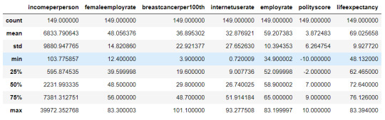
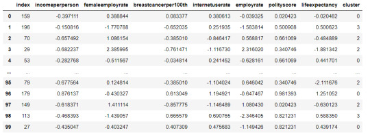
cluster = data_clean[['incomeperperson','femaleemployrate','breastcancerper100th','internetuserate', 'employrate', 'polityscore', 'lifeexpectancy']] cluster.describe()
#Standardize the clustering variables to have mean = 0 and standard deviation = 1
clustervar=cluster.copy() clustervar['incomeperperson']=preprocessing.scale(clustervar['incomeperperson'].astype('float64')) clustervar['femaleemployrate']=preprocessing.scale(clustervar['femaleemployrate'].astype('float64')) clustervar['breastcancerper100th']=preprocessing.scale(clustervar['breastcancerper100th'].astype('float64')) clustervar['internetuserate']=preprocessing.scale(clustervar['internetuserate'].astype('float64')) clustervar['employrate']=preprocessing.scale(clustervar['employrate'].astype('float64')) clustervar['polityscore']=preprocessing.scale(clustervar['polityscore'].astype('float64')) clustervar['lifeexpectancy']=preprocessing.scale(clustervar['lifeexpectancy'].astype('float64'))
#Split the data into train and test sets
clus_train, clus_test = train_test_split(clustervar, test_size=.3, random_state=123)
#Perform k-means cluster analysis for 1-9 clusters
from scipy.spatial.distance import cdist clusters = range(1,10) meandist = []
for k in clusters: model = KMeans(n_clusassign = k) model.fit(clus_train) clusters = model.predict(clus_train) meandist.append(sum(np.min(cdist(clus_train, model.cluster_centers_, 'euclidean'), axis=1)) / clus_train.shape[0])
#Plot average distance from observations from the cluster centroid to use the Elbow Method to identify number of clusters to choose
plt.plot(clusters, meandist) plt.xlabel('Number of clusters') plt.ylabel('Average distance') plt.title('Selecting k with the Elbow Method') plt.show()
#Interpret 3 cluster solution
model3 = KMeans(n_clusters=4) model3.fit(clus_train) clusassign = model3.predict(clus_train)
#Plot the clusters
from sklearn.decomposition import PCA pca_2 = PCA(2) plt.figure() plot_columns = pca_2.fit_transform(clus_train) plt.scatter(x=plot_columns[:,0], y=plot_columns[:,1], c=model3.labels_,) plt.xlabel('Canonical variable 1') plt.ylabel('Canonical variable 2') plt.title('Scatterplot of Canonical Variables for 4 Clusters') plt.show()
#Create a unique identifier variable from the index for the cluster training data to merge with the cluster assignment variable.
clus_train.reset_index(level=0, inplace=True)
#Create a list that has the new index variable
cluslist = list(clus_train['index'])
#Create a list of cluster assignments
labels = list(model3.labels_)
#Combine index variable list with cluster assignment list into a dictionary
newlist = dict(zip(cluslist, labels)) print(newlist)
#Convert newlist dictionary to a dataframe
newclus = pd.DataFrame.from_dict(newlist, orient='index')
#Rename the cluster assignment column
newclus.columns = ['cluster'] newclus
#Create a unique identifier variable from the index for the cluster assignment dataframe to merge with cluster training data
newclus.reset_index(level=0, inplace=True)
#Merge the cluster assignment dataframe with the cluster training variable dataframe by the index variable
merged_train = pd.merge(clus_train, newclus, on='index') merged_train.head(n=100)
#Cluster frequencies
merged_train.cluster.value_counts()

#Calculate clustering variable means by cluster
clustergrp = merged_train.groupby('cluster').mean() print ("Clustering variable means by cluster") clustergrp
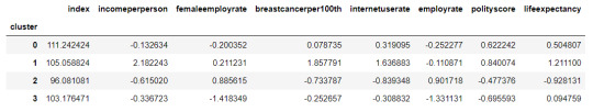
#Validate clusters in training data by examining cluster differences in urbanrate using ANOVA.
#First, merge urbanrate with clustering variables and cluster assignment data
urbanrate_data = data_clean['urbanrate']
#Split urbanrate data into train and test sets
urbanrate_train, internetuserate_test = train_test_split(urbanrate_data, test_size=.3, random_state=123) urbanrate_train1=pd.DataFrame(urbanrate_train) urbanrate_train1.reset_index(level=0, inplace=True) merged_train_all=pd.merge(urbanrate_train1, merged_train, on='index') sub5 = merged_train_all[['urbanrate', 'cluster']].dropna() urbanrate_mod = smf.ols(formula='urbanrate ~ C(cluster)', data=sub5).fit() urbanrate_mod.summary()
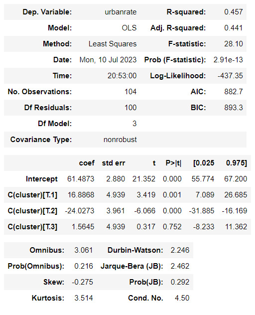
#Means for urbanrate by cluster
m1= sub5.groupby('cluster').mean() m1
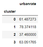
#Standard deviations for urbanrate by cluster
m2= sub5.groupby('cluster').std() m2
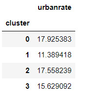
mc1 = multi.MultiComparison(sub5['urbanrate'], sub5['cluster']) res1 = mc1.tukeyhsd() res1.summary()
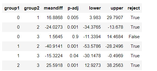
0 notes
Text
Código K- means craters of mars
-- coding: utf-8 --
""" Created on Fri Jun 16 19:08:39 2023
@author: ANGELA """ from pandas import Series, DataFrame import pandas import numpy as np import matplotlib.pylab as plt from sklearn.model_selection import train_test_split from sklearn import preprocessing from sklearn.cluster import KMeans
"""Data management"""
data = pandas.read_csv('marscrater_pds.csv', low_memory=False) data['LATITUDE_CIRCLE_IMAGE']=pandas.to_numeric(data['LATITUDE_CIRCLE_IMAGE'],errors='coerce') data['LONGITUDE_CIRCLE_IMAGE']=pandas.to_numeric(data['LONGITUDE_CIRCLE_IMAGE'],errors='coerce') data['DIAM_CIRCLE_IMAGE']=pandas.to_numeric(data['DIAM_CIRCLE_IMAGE'],errors='coerce') data['NUMBER_LAYERS']=pandas.to_numeric(data['NUMBER_LAYERS'],errors='coerce') data['DEPTH_RIMFLOOR_TOPOG']=pandas.to_numeric(data['DEPTH_RIMFLOOR_TOPOG'],errors='coerce')
upper-case all DataFrame column names
data.columns = map(str.upper, data.columns) data_clean =data.dropna()
target = data_clean.DEPTH_RIMFLOOR_TOPOG
select predictor variables and target variable as separate data sets
cluster= data_clean[['LATITUDE_CIRCLE_IMAGE','LONGITUDE_CIRCLE_IMAGE','DIAM_CIRCLE_IMAGE']] cluster.describe()
standardize clustering variables to have mean=0 and sd=1
clustervar=cluster.copy() clustervar['LATITUDE_CIRCLE_IMAGE']=preprocessing.scale(clustervar['LATITUDE_CIRCLE_IMAGE'].astype('float64')) clustervar['LONGITUDE_CIRCLE_IMAGE']=preprocessing.scale(clustervar['LONGITUDE_CIRCLE_IMAGE'].astype('float64')) clustervar['DIAM_CIRCLE_IMAGE']=preprocessing.scale(clustervar['DIAM_CIRCLE_IMAGE'].astype('float64'))
clustervar['DEPTH_RIMFLOOR_TOPOG']=preprocessing.scale(clustervar['DEPTH_RIMFLOOR_TOPOG'].astype('float64'))
split data into train and test sets
clus_train, clus_test = train_test_split(clustervar, test_size=.3, random_state=200)
k-means cluster analysis for 1-9 clusters
from scipy.spatial.distance import cdist clusters=range(1,10) meandist=[]
Calculate cluster
for k in clusters: model=KMeans(n_clusters=k) model.fit(clus_train) clusassign=model.predict(clus_train) meandist.append(sum(np.min(cdist(clus_train, model.cluster_centers_, 'euclidean'), axis=1)) / clus_train.shape[0])
""" Plot average distance from observations from the cluster centroid to use the Elbow Method to identify number of clusters to choose """
plt.plot(clusters, meandist) plt.xlabel('Number of clusters') plt.ylabel('Average distance') plt.title('Selecting k with the Elbow Method to date craters of mars')
Interpret 3 cluster solution
model3=KMeans(n_clusters=3) model3.fit(clus_train) clusassign=model3.predict(clus_train)
plot clusters
from sklearn.decomposition import PCA pca_2 = PCA(2) plot_columns = pca_2.fit_transform(clus_train) plt.scatter(x=plot_columns[:,0], y=plot_columns[:,1], c=model3.labels_,) plt.xlabel('Canonical variable 1') plt.ylabel('Canonical variable 2') plt.title('Scatterplot of Canonical Variables for 3 Clusters to date craters of mars') plt.show()
""" BEGIN multiple steps to merge cluster assignment with clustering variables to examine cluster variable means by cluster """
create a unique identifier variable from the index for the
cluster training data to merge with the cluster assignment variable
clus_train.reset_index(level=0, inplace=True)
create a list that has the new index variable
cluslist=list(clus_train['index'])
create a list of cluster assignments
labels=list(model3.labels_)
combine index variable list with cluster assignment list into a dictionary
newlist=dict(zip(cluslist, labels)) newlist
convert newlist dictionary to a dataframe
newclus=DataFrame.from_dict(newlist, orient='index') newclus
rename the cluster assignment column
newclus.columns = ['cluster']
now do the same for the cluster assignment variable
create a unique identifier variable from the index for the
cluster assignment dataframe
to merge with cluster training data
newclus.reset_index(level=0, inplace=True)
merge the cluster assignment dataframe with the cluster training variable dataframe
by the index variable
merged_train=pandas.merge(clus_train, newclus, on='index') merged_train.head(n=100)
cluster frequencies
merged_train.cluster.value_counts()
""" END multiple steps to merge cluster assignment with clustering variables to examine cluster variable means by cluster """
FINALLY calculate clustering variable means by cluster
clustergrp = merged_train.groupby('cluster').mean() print ("Clustering variable means by cluster") print(clustergrp)
validate clusters in training data by examining cluster differences in DEPTH_RIMFLOOR_TOPOG using ANOVA
first have to merge DEPTH_RIMFLOOR_TOPOG with clustering variables and cluster assignment data
DRT_data=data_clean['DEPTH_RIMFLOOR_TOPOG']
split DEPTH_RIMFLOOR_TOPOG data into train and test sets
DRT_train, DRT_test = train_test_split(DRT_data, test_size=.3, random_state=123) DRT_train1=pandas.DataFrame(DRT_train) DRT_train1.reset_index(level=0, inplace=True) merged_train_all=pandas.merge(DRT_train1, merged_train, on='index') sub1 = merged_train_all[['DEPTH_RIMFLOOR_TOPOG', 'cluster']].dropna()
import statsmodels.formula.api as smf import statsmodels.stats.multicomp as multi
DTRmod = smf.ols(formula='DEPTH_RIMFLOOR_TOPOG ~ C(cluster)', data=sub1).fit() print (DTRmod.summary())
print ('means for DEPTH_RIMFLOOR_TOPOG by cluster') m1= sub1.groupby('cluster').mean() print (m1)
print ('standard deviations for DEPTH_RIMFLOOR_TOPOG by cluster') m2= sub1.groupby('cluster').std() print (m2)
mc1 = multi.MultiComparison(sub1['GPA1'], sub1['cluster']) res1 = mc1.tukeyhsd() print(res1.summary())
Resultados
Los cluster posibles son 3, 5, 7 y 8 donde se evidencia un punto de quiebre en la ilustración, por lo que se realizó la prueba con 3 clusters y se evidencia que puede presentarse un overfiting al esta muy cerca y cobre puestos los clusters
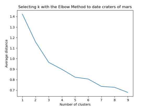
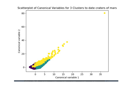
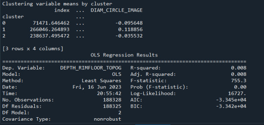

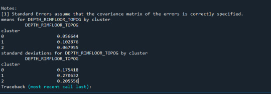
0 notes
Text
pyspark dataframe | python spark dataframe with examples
What is the pyspark dataframe?
How pyspark dataframe is evaluated?
Which is the entry point for pyspark?
How dataframes are created?
Can we Specify the schema of data as well while creating the dataframe?
Practical examples of how to create a dataframe using different data sources.
Example: converting the list of numeric into a pyspark dataframe.
Example: converting the tuple having employee details into a pyspark dataframe.
Example: converting the dictionary having a list of countries and their capitals into a pyspark dataframe.
Example: creating ‘pyspark.sql.rows’ object of number and their square and converting it into pyspark dataframe.
Example: creating python pandas dataframe and then converting the pandas dataframe into pyspark dataframe.
Example: converting the list of numbers into a pyspark dataframe by using pyspark RDD.
1. What is the pyspark dataframe?
A pyspark dataframe is equivalent to a table in a relational database, it is also equivalent to a data frame in Python/R. The pyspark dataframe comes with greater capabilities. We can also say that a dataframe is a dataset that is organized into named columns. You can create a pyspark dataframe from different sources like from python list/tuple/dictionary, using a relational database table, using existing RDD.
for complete article Please visit below url
https://mycloudplace.com/pyspark-dataframe-python-spark-dataframe-with-examples/
2 notes
·
View notes