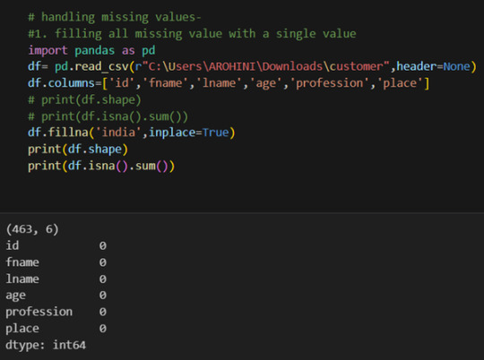
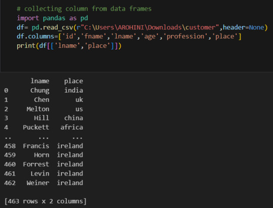
#select columns in pandas dataframe

[codewithnazam]

DataFrame in Pandas: Guide to Creating Awesome DataFrames

Explore how to create a dataframe in Pandas, including data input methods, customization options, and practical examples.

Data analysis used to be a daunting task, reserved for statisticians and mathematicians. But with the rise of powerful tools like Python and its fantastic library, Pandas, anyone can become a data whiz! Pandas, in particular, shines with its DataFrames, these nifty tables that organize and manipulate data like magic. But where do you start? Fear not, fellow data enthusiast, for this guide will…

[machinelearningcoursera]

K-mean Analysis

Script:

from pandas import Series, DataFrame import pandas as pd import numpy as np import matplotlib.pylab as plt from sklearn.model_selection import train_test_split from sklearn import preprocessing from sklearn.cluster import KMeans import os """ Data Management """

data = pd.read_csv("tree_addhealth.csv")

upper-case all DataFrame column names

data.columns = map(str.upper, data.columns)

Data Management

data_clean = data.dropna()

subset clustering variables

cluster=data_clean[['ALCEVR1','MAREVER1','ALCPROBS1','DEVIANT1','VIOL1', 'DEP1','ESTEEM1','SCHCONN1','PARACTV', 'PARPRES','FAMCONCT']] cluster.describe()

standardize clustering variables to have mean=0 and sd=1

clustervar=cluster.copy() clustervar['ALCEVR1']=preprocessing.scale(clustervar['ALCEVR1'].astype('float64')) clustervar['ALCPROBS1']=preprocessing.scale(clustervar['ALCPROBS1'].astype('float64')) clustervar['MAREVER1']=preprocessing.scale(clustervar['MAREVER1'].astype('float64')) clustervar['DEP1']=preprocessing.scale(clustervar['DEP1'].astype('float64')) clustervar['ESTEEM1']=preprocessing.scale(clustervar['ESTEEM1'].astype('float64')) clustervar['VIOL1']=preprocessing.scale(clustervar['VIOL1'].astype('float64')) clustervar['DEVIANT1']=preprocessing.scale(clustervar['DEVIANT1'].astype('float64')) clustervar['FAMCONCT']=preprocessing.scale(clustervar['FAMCONCT'].astype('float64')) clustervar['SCHCONN1']=preprocessing.scale(clustervar['SCHCONN1'].astype('float64')) clustervar['PARACTV']=preprocessing.scale(clustervar['PARACTV'].astype('float64')) clustervar['PARPRES']=preprocessing.scale(clustervar['PARPRES'].astype('float64'))

split data into train and test sets

clus_train, clus_test = train_test_split(clustervar, test_size=.3, random_state=123)

k-means cluster analysis for 1-9 clusters

from scipy.spatial.distance import cdist clusters=range(1,9) meandist=[]

for k in clusters: model=KMeans(n_clusters=k) model.fit(clus_train) clusassign=model.predict(clus_train) meandist.append(sum(np.min(cdist(clus_train, model.cluster_centers_, 'euclidean'), axis=1)) / clus_train.shape[0])

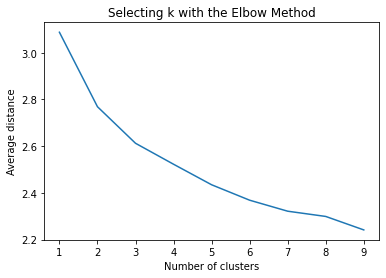
""" Plot average distance from observations from the cluster centroid to use the Elbow Method to identify number of clusters to choose """

plt.plot(clusters, meandist) plt.xlabel('Number of clusters') plt.ylabel('Average distance') plt.title('Selecting k with the Elbow Method')

Interpret 3 cluster solution

model3=KMeans(n_clusters=2) model3.fit(clus_train) clusassign=model3.predict(clus_train)

plot clusters

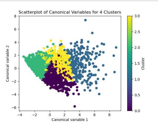
from sklearn.decomposition import PCA pca_2 = PCA(2) plot_columns = pca_2.fit_transform(clus_train) plt.scatter(x=plot_columns[:,0], y=plot_columns[:,1], c=model3.labels_) plt.xlabel('Canonical variable 1') plt.ylabel('Canonical variable 2') plt.title('Scatterplot of Canonical Variables for 4 Clusters')

Add the legend to the plot

import matplotlib.patches as mpatches patches = [mpatches.Patch(color=plt.cm.viridis(i/4), label=f'Cluster {i}') for i in range(4)]

plt.legend(handles=patches, title="Clusters") plt.show()

""" BEGIN multiple steps to merge cluster assignment with clustering variables to examine cluster variable means by cluster """

create a unique identifier variable from the index for the

cluster training data to merge with the cluster assignment variable

clus_train.reset_index(level=0, inplace=True)

create a list that has the new index variable

cluslist=list(clus_train['index'])

create a list of cluster assignments

labels=list(model3.labels_)

combine index variable list with cluster assignment list into a dictionary

newlist=dict(zip(cluslist, labels)) newlist

convert newlist dictionary to a dataframe

newclus=DataFrame.from_dict(newlist, orient='index') newclus

rename the cluster assignment column

newclus.columns = ['cluster']

now do the same for the cluster assignment variable

create a unique identifier variable from the index for the

cluster assignment dataframe

to merge with cluster training data

newclus.reset_index(level=0, inplace=True)

merge the cluster assignment dataframe with the cluster training variable dataframe

by the index variable

merged_train=pd.merge(clus_train, newclus, on='index') merged_train.head(n=100)

cluster frequencies

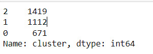
merged_train.cluster.value_counts()

""" END multiple steps to merge cluster assignment with clustering variables to examine cluster variable means by cluster """

FINALLY calculate clustering variable means by cluster

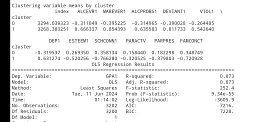
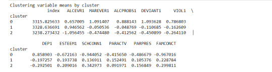
clustergrp = merged_train.groupby('cluster').mean() print ("Clustering variable means by cluster") print(clustergrp)

validate clusters in training data by examining cluster differences in GPA using ANOVA

first have to merge GPA with clustering variables and cluster assignment data

gpa_data=data_clean['GPA1']

split GPA data into train and test sets

gpa_train, gpa_test = train_test_split(gpa_data, test_size=.3, random_state=123) gpa_train1=pd.DataFrame(gpa_train) gpa_train1.reset_index(level=0, inplace=True) merged_train_all=pd.merge(gpa_train1, merged_train, on='index') sub1 = merged_train_all[['GPA1', 'cluster']].dropna()

import statsmodels.formula.api as smf import statsmodels.stats.multicomp as multi

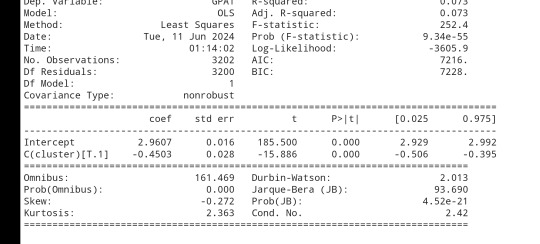
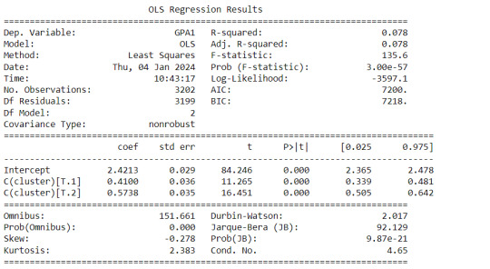
gpamod = smf.ols(formula='GPA1 ~ C(cluster)', data=sub1).fit() print (gpamod.summary())

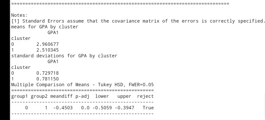
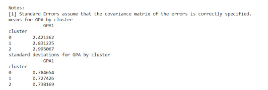
print ('means for GPA by cluster') m1= sub1.groupby('cluster').mean() print (m1)

print ('standard deviations for GPA by cluster') m2= sub1.groupby('cluster').std() print (m2)

mc1 = multi.MultiComparison(sub1['GPA1'], sub1['cluster']) res1 = mc1.tukeyhsd() print(res1.summary())

------------------------------------------------------------------------------

PLOTS:

------------------------------------------------------------------------------ANALYSING:

The K-mean cluster analysis is trying to identify subgroups of adolescents based on their similarity using the following 11 variables:

(Binary variables)

ALCEVR1 = ever used alcohol

MAREVER1 = ever used marijuana

(Quantitative variables)

ALCPROBS1 = Alcohol problem

DEVIANT1 = behaviors scale

VIOL1 = Violence scale

DEP1 = depression scale

ESTEEM1 = Self-esteem

SCHCONN1= School connectiveness

PARACTV = parent activities

PARPRES = parent presence

FAMCONCT = family connectiveness

The test was split with 70% for the training set and 30% for the test set. 9 clusters were conducted and the results are shown the plot 1. The plot suggest 2,4 , 5 and 6 solutions might be interpreted.

The second plot shows the canonical discriminant analyses of the 4 cluster solutions. Clusters 0 and 3 are very densely packed together with relatively low within-cluster variance whereas clusters 1 and 2 were spread out more than the other clusters, especially cluster 1 which means there is higher variance within the cluster. The number of clusters we would need to use is less the 3.

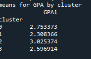
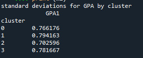
Students in cluster 2 had higher GPA values with an SD of 0.70 and cluster 1 had lower GPA values with an SD of 0.79

[usesofcannabis]

Generating a Correlation Coefficient

This assignment aims to statistically assess the evidence, provided by NESARC codebook, in favor of or against the association between cannabis use and mental illnesses, such as major depression and general anxiety, in U.S. adults. More specifically, since my research question includes only categorical variables, I selected three new quantitative variables from the NESARC codebook. Therefore, I redefined my hypothesis and examined the correlation between the age when the individuals began using cannabis the most (quantitative explanatory, variable “S3BD5Q2F”) and the age when they experienced the first episode of major depression and general anxiety (quantitative response, variables “S4AQ6A” and ”S9Q6A”). As a result, in the first place, in order to visualize the association between cannabis use and both depression and anxiety episodes, I used seaborn library to produce a scatterplot for each disorder separately and interpreted the overall patterns, by describing the direction, as well as the form and the strength of the relationships. In addition, I ran Pearson correlation test (Q->Q) twice (once for each disorder) and measured the strength of the relationships between each pair of quantitative variables, by numerically generating both the correlation coefficients r and the associated p-values. For the code and the output I used Spyder (IDE).

The three quantitative variables that I used for my Pearson correlation tests are:

  

FOLLWING IS A PYTHON PROGRAM TO CALCULATE CORRELATION

import pandas import numpy import seaborn import scipy import matplotlib.pyplot as plt

nesarc = pandas.read_csv ('nesarc_pds.csv' , low_memory=False)

Set PANDAS to show all columns in DataFrame

pandas.set_option('display.max_columns', None)

Set PANDAS to show all rows in DataFrame

pandas.set_option('display.max_rows', None)

nesarc.columns = map(str.upper , nesarc.columns)

pandas.set_option('display.float_format' , lambda x:'%f'%x)

Change my variables to numeric

nesarc['AGE'] = pandas.to_numeric(nesarc['AGE'], errors='coerce') nesarc['S3BQ4'] = pandas.to_numeric(nesarc['S3BQ4'], errors='coerce') nesarc['S4AQ6A'] = pandas.to_numeric(nesarc['S4AQ6A'], errors='coerce') nesarc['S3BD5Q2F'] = pandas.to_numeric(nesarc['S3BD5Q2F'], errors='coerce') nesarc['S9Q6A'] = pandas.to_numeric(nesarc['S9Q6A'], errors='coerce') nesarc['S4AQ7'] = pandas.to_numeric(nesarc['S4AQ7'], errors='coerce') nesarc['S3BQ1A5'] = pandas.to_numeric(nesarc['S3BQ1A5'], errors='coerce')

Subset my sample

subset1 = nesarc[(nesarc['S3BQ1A5']==1)] # Cannabis users subsetc1 = subset1.copy()

Setting missing data

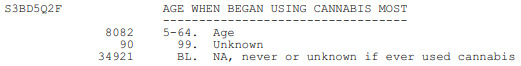
subsetc1['S3BQ1A5']=subsetc1['S3BQ1A5'].replace(9, numpy.nan) subsetc1['S3BD5Q2F']=subsetc1['S3BD5Q2F'].replace('BL', numpy.nan) subsetc1['S3BD5Q2F']=subsetc1['S3BD5Q2F'].replace(99, numpy.nan) subsetc1['S4AQ6A']=subsetc1['S4AQ6A'].replace('BL', numpy.nan) subsetc1['S4AQ6A']=subsetc1['S4AQ6A'].replace(99, numpy.nan) subsetc1['S9Q6A']=subsetc1['S9Q6A'].replace('BL', numpy.nan) subsetc1['S9Q6A']=subsetc1['S9Q6A'].replace(99, numpy.nan)

Scatterplot for the age when began using cannabis the most and the age of first episode of major depression

plt.figure(figsize=(12,4)) # Change plot size scat1 = seaborn.regplot(x="S3BD5Q2F", y="S4AQ6A", fit_reg=True, data=subset1) plt.xlabel('Age when began using cannabis the most') plt.ylabel('Age when expirenced the first episode of major depression') plt.title('Scatterplot for the age when began using cannabis the most and the age of first the episode of major depression') plt.show()

data_clean=subset1.dropna()

Pearson correlation coefficient for the age when began using cannabis the most and the age of first the episode of major depression

print ('Association between the age when began using cannabis the most and the age of the first episode of major depression') print (scipy.stats.pearsonr(data_clean['S3BD5Q2F'], data_clean['S4AQ6A']))

Scatterplot for the age when began using cannabis the most and the age of the first episode of general anxiety

plt.figure(figsize=(12,4)) # Change plot size scat2 = seaborn.regplot(x="S3BD5Q2F", y="S9Q6A", fit_reg=True, data=subset1) plt.xlabel('Age when began using cannabis the most') plt.ylabel('Age when expirenced the first episode of general anxiety') plt.title('Scatterplot for the age when began using cannabis the most and the age of the first episode of general anxiety') plt.show()

Pearson correlation coefficient for the age when began using cannabis the most and the age of the first episode of general anxiety

print ('Association between the age when began using cannabis the most and the age of first the episode of general anxiety') print (scipy.stats.pearsonr(data_clean['S3BD5Q2F'], data_clean['S9Q6A']))

OUTPUT:

The scatterplot presented above, illustrates the correlation between the age when individuals began using cannabis the most (quantitative explanatory variable) and the age when they experienced the first episode of depression (quantitative response variable). The direction of the relationship is positive (increasing), which means that an increase in the age of cannabis use is associated with an increase in the age of the first depression episode. In addition, since the points are scattered about a line, the relationship is linear. Regarding the strength of the relationship, from the pearson correlation test we can see that the correlation coefficient is equal to 0.23, which indicates a weak linear relationship between the two quantitative variables. The associated p-value is equal to 2.27e-09 (p-value is written in scientific notation) and the fact that its is very small means that the relationship is statistically significant. As a result, the association between the age when began using cannabis the most and the age of the first depression episode is moderately weak, but it is highly unlikely that a relationship of this magnitude would be due to chance alone. Finally, by squaring the r, we can find the fraction of the variability of one variable that can be predicted by the other, which is fairly low at 0.05.

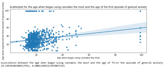
For the association between the age when individuals began using cannabis the most (quantitative explanatory variable) and the age when they experienced the first episode of anxiety (quantitative response variable), the scatterplot psented above shows a positive linear relationship. Regarding the strength of the relationship, the pearson correlation test indicates that the correlation coefficient is equal to 0.14, which is interpreted to a fairly weak linear relationship between the two quantitative variables. The associated p-value is equal to 0.0001, which means that the relationship is statistically significant. Therefore, the association between the age when began using cannabis the most and the age of the first anxiety episode is weak, but it is highly unlikely that a relationship of this magnitude would be due to chance alone. Finally, by squaring the r, we can find the fraction of the variability of one variable that can be predicted by the other, which is very low at 0.01.

[analyticsshiksha30]

What is Pandas in Data analysis

Pandas in data analysis is a popular Python library specifically designed for data manipulation and analysis. It provides high-performance, easy-to-use data structures and tools, making it essential for handling structured data in pandas data analysis. Pandas is built on top of NumPy, offering a more flexible and powerful framework for working with datasets.

Pandas revolve­s around two primary structures, Series (a single­ line of data) and DataFrame (a grid of data). Imagine a DataFrame­ as a table or a spreadshee­t. It offers a place to hold and tweak table­-like data, with rows acting as individual entries and columns standing for characte­ristics.

The Pandas library simplifies the process of reading, cleaning, and modifying data from different formats like­ CSV, Excel, JSON, and SQL databases. It provides numerous built-in functions for handling missing data, merging datasets, and reshaping data, which are essential tasks in data preprocessing.

Additionally, Pandas supports filtering, selecting, and sorting data efficiently, helping analysts perform complex operations with just a few lines of code. Its ability to group, aggregate, and summarize data makes it easy to calculate key statistics or extract meaningful insights.

Pandas also integrates with data visualization libraries like Matplotlib, making it a comprehensive tool for data analysis, data wrangling, and visualization, used by data scientists, analysts, and engineers.

[mengchunhsieh]

K-means clusthering

#importamos las librerías necesarias

from pandas import Series,DataFrame

import pandas as pd

import numpy as np

import matplotlib.pylab as plt

from sklearn.model_selection

import train_test_splitfrom sklearn

import preprocessing

from sklearn.cluster import KMeans

"""Data Management"""

data =pd.read_csv("/content/drive/MyDrive/tree_addhealth.csv" )

#upper-case all DataFrame column names

data.columns = map(str.upper, data.columns)

# Data Managementdata_clean = data.dropna()

# subset clustering variablescluster=data_clean[['ALCEVR1','MAREVER1','ALCPROBS1','DEVIANT1','VIOL1','DEP1','ESTEEM1','SCHCONN1','PARACTV', 'PARPRES','FAMCONCT']]

cluster.describe()

# standardize clustering variables to have mean=0 and sd=1

clustervar=cluster.copy()

clustervar['ALCEVR1']=preprocessing.scale(clustervar['ALCEVR1'].astype('float64'))

clustervar['ALCPROBS1']=preprocessing.scale(clustervar['ALCPROBS1'].astype('float64'))

clustervar['MAREVER1']=preprocessing.scale(clustervar['MAREVER1'].astype('float64'))

clustervar['DEP1']=preprocessing.scale(clustervar['DEP1'].astype('float64'))

clustervar['ESTEEM1']=preprocessing.scale(clustervar['ESTEEM1'].astype('float64'))

clustervar['VIOL1']=preprocessing.scale(clustervar['VIOL1'].astype('float64'))

clustervar['DEVIANT1']=preprocessing.scale(clustervar['DEVIANT1'].astype('float64'))

clustervar['FAMCONCT']=preprocessing.scale(clustervar['FAMCONCT'].astype('float64'))

clustervar['SCHCONN1']=preprocessing.scale(clustervar['SCHCONN1'].astype('float64'))

clustervar['PARACTV']=preprocessing.scale(clustervar['PARACTV'].astype('float64'))

clustervar['PARPRES']=preprocessing.scale(clustervar['PARPRES'].astype('float64'))

# split data into train and test sets

clus_train, clus_test = train_test_split(clustervar, test_size=.3, random_state=123)

# k-means cluster analysis for 1-9 clusters

from scipy.spatial.distance import cdist

clusters=range(1,10)

meandist=[]

for k in clusters: model=KMeans(n_clusters=k) model.fit(clus_train) clusassign=model.predict(clus_train) meandist.append(sum(np.min(cdist(clus_train, model.cluster_centers_, 'euclidean'), axis=1))

/ clus_train.shape[0])

"""Plot average distance from observations from the cluster centroidto use the Elbow Method to identify number of clusters to choose"""

plt.plot(clusters,meandist)

plt.xlabel('Number of clusters')

plt.ylabel('Average distance')

plt.title('Selecting k with the Elbow Method')

# Interpret 2 cluster solution

model2=KMeans(n_clusters=2)model2.fit(clus_train)

clusassign=model2.predict(clus_train)

# plot clusters

from sklearn.decomposition import PCA

pca_2 = PCA(2)

plot_columns = pca_2.fit_transform(clus_train)

plt.scatter(x=plot_columns[:,0],y=plot_columns[:,1],c=model2.labels_,)

plt.xlabel('Canonical variable 1')

plt.ylabel('Canonical variable 2')

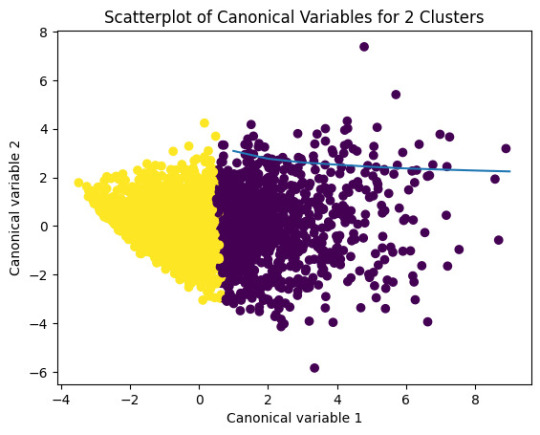
plt.title('Scatterplot of Canonical Variables for 2 Clusters')

plt.show()

"""BEGIN multiple steps to merge cluster assignment with clustering variables to examinecluster variable means by cluster"""

# create a unique identifier variable from the index for the

# cluster training data to merge with the cluster assignment variable

clus_train.reset_index(level=0, inplace=True)

# create a list that has the new index variable

cluslist=list(clus_train['index'])

# create a list of cluster assignments

labels=list(model2.labels_)

# combine index variable list with cluster assignment list into a dictionary

newlist=dict(zip(cluslist, labels))newlist

# convert newlist dictionary to a dataframenew

clus=DataFrame.from_dict(newlist, orient='index')newclus

# rename the cluster assignment columnnew

clus.columns = ['cluster']

# now do the same for the cluster assignment variable

# create a unique identifier variable from the index for the

# cluster assignment dataframe

# to merge with cluster training datanew

clus.reset_index(level=0, inplace=True)

# merge the cluster assignment dataframe with the cluster training variable dataframe

# by the index variablemerged_train=pd.merge(clus_train, newclus, on='index')

merged_train.head(n=100)

# cluster frequenciesmerged_train.cluster.value_counts()

"""END multiple steps to merge cluster assignment with clustering variables to examinecluster variable means by cluster"""

# FINALLY calculate clustering variable means by

clusterclustergrp = merged_train.groupby('cluster').mean()print ("Clustering variable means by cluster")

print(clustergrp)

# validate clusters in training data by examining cluster differences in GPA using ANOVA

# first have to merge GPA with clustering variables and cluster assignment data

gpa_data=data_clean['GPA1']

# split GPA data into train and test sets

gpa_train, gpa_test = train_test_split(gpa_data, test_size=.3, random_state=123)

gpa_train1=pd.DataFrame(gpa_train)

gpa_train1.reset_index(level=0, inplace=True)

merged_train_all=pd.merge(gpa_train1, merged_train, on='index')

sub1 = merged_train_all[['GPA1', 'cluster']].dropna()

import statsmodels.formula.api as smf

import statsmodels.stats.multicomp as multi

gpamod = smf.ols(formula='GPA1 ~ C(cluster)', data=sub1).fit()

print (gpamod.summary())

print ('means for GPA by cluster')

m1= sub1.groupby('cluster').mean()

print (m1)

print ('standard deviations for GPA by cluster')

m2= sub1.groupby('cluster').std()print (m2)

mc1 = multi.MultiComparison(sub1['GPA1'], sub1['cluster'])

res1 = mc1.tukeyhsd()

print(res1.summary())

爆發

0 則迴響

[rogerscode]

K-means clusthering

#importamos las librerías necesarias

from pandas import Series,DataFrame

import pandas as pd

import numpy as np

import matplotlib.pylab as plt

from sklearn.model_selection

import train_test_splitfrom sklearn

import preprocessing

from sklearn.cluster import KMeans

"""Data Management"""

data =pd.read_csv("/content/drive/MyDrive/tree_addhealth.csv" )

#upper-case all DataFrame column names

data.columns = map(str.upper, data.columns)

# Data Managementdata_clean = data.dropna()

# subset clustering variablescluster=data_clean[['ALCEVR1','MAREVER1','ALCPROBS1','DEVIANT1','VIOL1','DEP1','ESTEEM1','SCHCONN1','PARACTV', 'PARPRES','FAMCONCT']]

cluster.describe()

# standardize clustering variables to have mean=0 and sd=1

clustervar=cluster.copy()

clustervar['ALCEVR1']=preprocessing.scale(clustervar['ALCEVR1'].astype('float64'))

clustervar['ALCPROBS1']=preprocessing.scale(clustervar['ALCPROBS1'].astype('float64'))

clustervar['MAREVER1']=preprocessing.scale(clustervar['MAREVER1'].astype('float64'))

clustervar['DEP1']=preprocessing.scale(clustervar['DEP1'].astype('float64'))

clustervar['ESTEEM1']=preprocessing.scale(clustervar['ESTEEM1'].astype('float64'))

clustervar['VIOL1']=preprocessing.scale(clustervar['VIOL1'].astype('float64'))

clustervar['DEVIANT1']=preprocessing.scale(clustervar['DEVIANT1'].astype('float64'))

clustervar['FAMCONCT']=preprocessing.scale(clustervar['FAMCONCT'].astype('float64'))

clustervar['SCHCONN1']=preprocessing.scale(clustervar['SCHCONN1'].astype('float64'))

clustervar['PARACTV']=preprocessing.scale(clustervar['PARACTV'].astype('float64'))

clustervar['PARPRES']=preprocessing.scale(clustervar['PARPRES'].astype('float64'))

# split data into train and test sets

clus_train, clus_test = train_test_split(clustervar, test_size=.3, random_state=123)

# k-means cluster analysis for 1-9 clusters

from scipy.spatial.distance import cdist

clusters=range(1,10)

meandist=[]

for k in clusters: model=KMeans(n_clusters=k) model.fit(clus_train) clusassign=model.predict(clus_train) meandist.append(sum(np.min(cdist(clus_train, model.cluster_centers_, 'euclidean'), axis=1))

/ clus_train.shape[0])

"""Plot average distance from observations from the cluster centroidto use the Elbow Method to identify number of clusters to choose"""

plt.plot(clusters,meandist)

plt.xlabel('Number of clusters')

plt.ylabel('Average distance')

plt.title('Selecting k with the Elbow Method')

# Interpret 2 cluster solution

model2=KMeans(n_clusters=2)model2.fit(clus_train)

clusassign=model2.predict(clus_train)

# plot clusters

from sklearn.decomposition import PCA

pca_2 = PCA(2)

plot_columns = pca_2.fit_transform(clus_train)

plt.scatter(x=plot_columns[:,0],y=plot_columns[:,1],c=model2.labels_,)

plt.xlabel('Canonical variable 1')

plt.ylabel('Canonical variable 2')

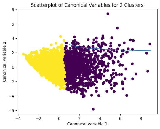
plt.title('Scatterplot of Canonical Variables for 2 Clusters')

plt.show()

"""BEGIN multiple steps to merge cluster assignment with clustering variables to examinecluster variable means by cluster"""

# create a unique identifier variable from the index for the

# cluster training data to merge with the cluster assignment variable

clus_train.reset_index(level=0, inplace=True)

# create a list that has the new index variable

cluslist=list(clus_train['index'])

# create a list of cluster assignments

labels=list(model2.labels_)

# combine index variable list with cluster assignment list into a dictionary

newlist=dict(zip(cluslist, labels))newlist

# convert newlist dictionary to a dataframenew

clus=DataFrame.from_dict(newlist, orient='index')newclus

# rename the cluster assignment columnnew

clus.columns = ['cluster']

# now do the same for the cluster assignment variable

# create a unique identifier variable from the index for the

# cluster assignment dataframe

# to merge with cluster training datanew

clus.reset_index(level=0, inplace=True)

# merge the cluster assignment dataframe with the cluster training variable dataframe

# by the index variablemerged_train=pd.merge(clus_train, newclus, on='index')

merged_train.head(n=100)

# cluster frequenciesmerged_train.cluster.value_counts()

"""END multiple steps to merge cluster assignment with clustering variables to examinecluster variable means by cluster"""

# FINALLY calculate clustering variable means by

clusterclustergrp = merged_train.groupby('cluster').mean()print ("Clustering variable means by cluster")

print(clustergrp)

# validate clusters in training data by examining cluster differences in GPA using ANOVA

# first have to merge GPA with clustering variables and cluster assignment data

gpa_data=data_clean['GPA1']

# split GPA data into train and test sets

gpa_train, gpa_test = train_test_split(gpa_data, test_size=.3, random_state=123)

gpa_train1=pd.DataFrame(gpa_train)

gpa_train1.reset_index(level=0, inplace=True)

merged_train_all=pd.merge(gpa_train1, merged_train, on='index')

sub1 = merged_train_all[['GPA1', 'cluster']].dropna()

import statsmodels.formula.api as smf

import statsmodels.stats.multicomp as multi

gpamod = smf.ols(formula='GPA1 ~ C(cluster)', data=sub1).fit()

print (gpamod.summary())

print ('means for GPA by cluster')

m1= sub1.groupby('cluster').mean()

print (m1)

print ('standard deviations for GPA by cluster')

m2= sub1.groupby('cluster').std()print (m2)

mc1 = multi.MultiComparison(sub1['GPA1'], sub1['cluster'])

res1 = mc1.tukeyhsd()

print(res1.summary())

[asquaretechnologies]

Beginner’s Guide: Data Analysis with Pandas

Data analysis is the process of sorting through all the data, looking for patterns, connections, and interesting things. It helps us make sense of information and use it to make decisions or find solutions to problems. When it comes to data analysis and manipulation in Python, the Pandas library reigns supreme. Pandas provide powerful tools for working with structured data, making it an indispensable asset for both beginners and experienced data scientists.

What is Pandas?

Pandas is an open-source Python library for data manipulation and analysis. It is built on top of NumPy, another popular numerical computing library, and offers additional features specifically tailored for data manipulation and analysis. There are two primary data structures in Pandas:

• Series: A one-dimensional array capable of holding any type of data.

• DataFrame: A two-dimensional labeled data structure similar to a table in relational databases.

It allows us to efficiently process and analyze data, whether it comes from any file types like CSV files, Excel spreadsheets, SQL databases, etc.

How to install Pandas?

We can install Pandas using the pip command. We can run the following codes in the terminal.

After installing, we can import it using:

How to load an external dataset using Pandas?

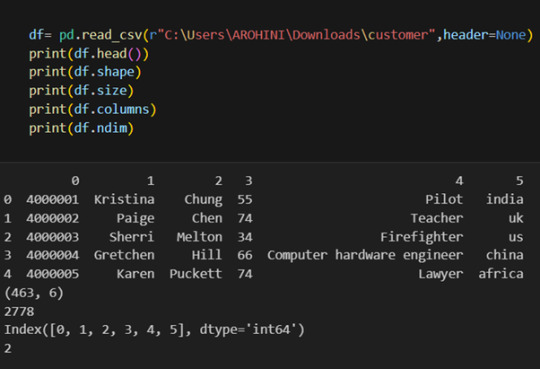
Pandas provide various functions for loading data into a data frame. One of the most commonly used functions is pd.read_csv() for reading CSV files. For example:

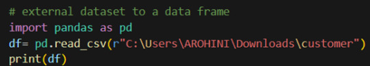
The output of the above code is:

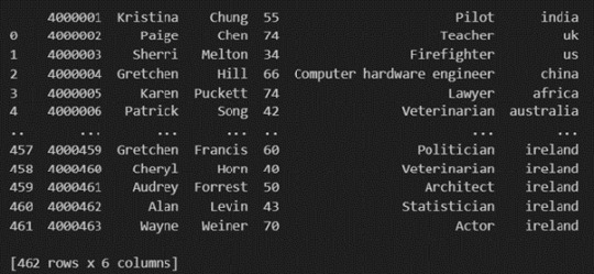
Once your data is loaded into a data frame, you can start exploring it. Pandas offers numerous methods and attributes for getting insights into your data. Here are a few examples:

df.head(): View the first few rows of the DataFrame.

df.tail(): View the last few rows of the DataFrame.

http://df.info(): Get a concise summary of the DataFrame, including data types and missing values.

df.describe(): Generate descriptive statistics for numerical columns.

df.shape: Get the dimensions of the DataFrame (rows, columns).

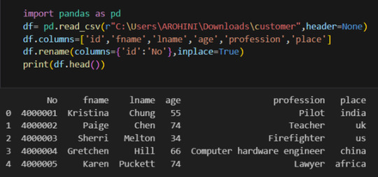
df.columns: Access the column labels of the DataFrame.

df.dtypes: Get the data types of each column.

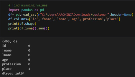
In data analysis, it is essential to do data cleaning. Pandas provide powerful tools for handling missing data, removing duplicates, and transforming data. Some common data-cleaning tasks include:

Handling missing values using methods like df.dropna() or df.fillna().

Removing duplicate rows with df.drop_duplicates().

Data type conversion using df.astype().

Renaming columns with df.rename().

Pandas excels in data manipulation tasks such as selecting subsets of data, filtering rows, and creating new columns. Here are a few examples:

Selecting columns: df[‘column_name’] or df[[‘column1’, ‘column2’]].

Filtering rows based on conditions: df[df[‘column’] > value].

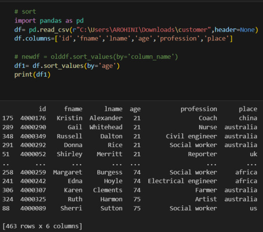
Sorting data: df.sort_values(by=’column’).

Grouping data: df.groupby(‘column’).mean().

With data cleaned and prepared, you can use Pandas to perform various analyses. Whether you’re computing statistics, performing exploratory data analysis, or building predictive models, Pandas provides the tools you need. Additionally, Pandas integrates seamlessly with other libraries such as Matplotlib and Seaborn for data visualization

[deba1407]

KMeans Clustering Assignment

Import the modules

from pandas import Series, DataFrame import pandas as pd import numpy as np import matplotlib.pylab as plt from sklearn.model_selection import train_test_split from sklearn import preprocessing from sklearn.cluster import KMeans

Load the dataset

data = pd.read_csv("C:\Users\guy3404\OneDrive - MDLZ\Documents\Cross Functional Learning\AI COP\Coursera\machine_learning_data_analysis\Datasets\tree_addhealth.csv")

data.head()

upper-case all DataFrame column names

data.columns = map(str.upper, data.columns)

Data Management

data_clean = data.dropna() data_clean.head()

subset clustering variables

cluster=data_clean[['ALCEVR1','MAREVER1','ALCPROBS1','DEVIANT1','VIOL1', 'DEP1','ESTEEM1','SCHCONN1','PARACTV', 'PARPRES','FAMCONCT']] cluster.describe()

standardize clustering variables to have mean=0 and sd=1

clustervar=cluster.copy() clustervar['ALCEVR1']=preprocessing.scale(clustervar['ALCEVR1'].astype('float64')) clustervar['ALCPROBS1']=preprocessing.scale(clustervar['ALCPROBS1'].astype('float64')) clustervar['MAREVER1']=preprocessing.scale(clustervar['MAREVER1'].astype('float64')) clustervar['DEP1']=preprocessing.scale(clustervar['DEP1'].astype('float64')) clustervar['ESTEEM1']=preprocessing.scale(clustervar['ESTEEM1'].astype('float64')) clustervar['VIOL1']=preprocessing.scale(clustervar['VIOL1'].astype('float64')) clustervar['DEVIANT1']=preprocessing.scale(clustervar['DEVIANT1'].astype('float64')) clustervar['FAMCONCT']=preprocessing.scale(clustervar['FAMCONCT'].astype('float64')) clustervar['SCHCONN1']=preprocessing.scale(clustervar['SCHCONN1'].astype('float64')) clustervar['PARACTV']=preprocessing.scale(clustervar['PARACTV'].astype('float64')) clustervar['PARPRES']=preprocessing.scale(clustervar['PARPRES'].astype('float64'))

split data into train and test sets

clus_train, clus_test = train_test_split(clustervar, test_size=.3, random_state=123)

k-means cluster analysis for 1-9 clusters

from scipy.spatial.distance import cdist clusters=range(1,10) meandist=[]

for k in clusters: model=KMeans(n_clusters=k) model.fit(clus_train) clusassign=model.predict(clus_train) meandist.append(sum(np.min(cdist(clus_train, model.cluster_centers_, 'euclidean'), axis=1)) / clus_train.shape[0])

""" Plot average distance from observations from the cluster centroid to use the Elbow Method to identify number of clusters to choose """ plt.plot(clusters, meandist) plt.xlabel('Number of clusters') plt.ylabel('Average distance') plt.title('Selecting k with the Elbow Method')

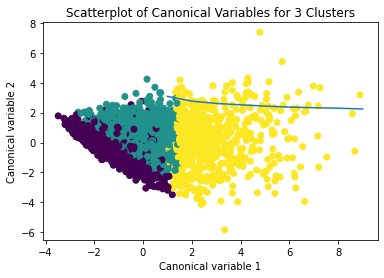
Interpret 3 cluster solution

model3=KMeans(n_clusters=3) model3.fit(clus_train) clusassign=model3.predict(clus_train)

plot clusters

from sklearn.decomposition import PCA pca_2 = PCA(2) plot_columns = pca_2.fit_transform(clus_train) plt.scatter(x=plot_columns[:,0], y=plot_columns[:,1], c=model3.labels_,) plt.xlabel('Canonical variable 1') plt.ylabel('Canonical variable 2') plt.title('Scatterplot of Canonical Variables for 3 Clusters') plt.show()

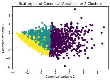
The datapoints of the 2 clusters in the left are less spread out but have more overlaps. The cluster to the right is more distinct but has more spread in the data points

""" BEGIN multiple steps to merge cluster assignment with clustering variables to examine cluster variable means by cluster """

create a unique identifier variable from the index for the

cluster training data to merge with the cluster assignment variable

clus_train.reset_index(level=0, inplace=True)

create a list that has the new index variable

cluslist=list(clus_train['index'])

create a list of cluster assignments

labels=list(model3.labels_)

combine index variable list with cluster assignment list into a dictionary

newlist=dict(zip(cluslist, labels)) newlist

convert newlist dictionary to a dataframe

newclus=DataFrame.from_dict(newlist, orient='index') newclus

rename the cluster assignment column

newclus.columns = ['cluster']

now do the same for the cluster assignment variable

create a unique identifier variable from the index for the

cluster assignment dataframe

to merge with cluster training data

newclus.reset_index(level=0, inplace=True)

merge the cluster assignment dataframe with the cluster training variable dataframe

by the index variable

merged_train=pd.merge(clus_train, newclus, on='index') merged_train.head(n=100)

cluster frequencies

merged_train.cluster.value_counts()

""" END multiple steps to merge cluster assignment with clustering variables to examine cluster variable means by cluster """

FINALLY calculate clustering variable means by cluster

clustergrp = merged_train.groupby('cluster').mean() print ("Clustering variable means by cluster") print(clustergrp)

validate clusters in training data by examining cluster differences in GPA using ANOVA

first have to merge GPA with clustering variables and cluster assignment data

gpa_data=data_clean['GPA1']

split GPA data into train and test sets

gpa_train, gpa_test = train_test_split(gpa_data, test_size=.3, random_state=123) gpa_train1=pd.DataFrame(gpa_train) gpa_train1.reset_index(level=0, inplace=True) merged_train_all=pd.merge(gpa_train1, merged_train, on='index') sub1 = merged_train_all[['GPA1', 'cluster']].dropna()

Print statistical summary by cluster

import statsmodels.formula.api as smf import statsmodels.stats.multicomp as multi

gpamod = smf.ols(formula='GPA1 ~ C(cluster)', data=sub1).fit() print (gpamod.summary())

print ('means for GPA by cluster') m1= sub1.groupby('cluster').mean() print (m1)

print ('standard deviations for GPA by cluster') m2= sub1.groupby('cluster').std() print (m2)

Interpretation

The clustering average summary shows Cluster 0 has higher alcohol and marijuana problems, shows higher deviant and violent behavior, suffers from depression, has low self esteem,school connectedness, paraental and family connectedness. On the contrary, Cluster 2 shows the lowest alcohol and marijuana problems, lowest deviant & violent behavior,depression, and higher self esteem,school connectedness, paraental and family connectedness. Further, when validated against GPA score, we observe Cluster 0 shows the lowest average GPA and CLuster 2 has the highest average GPA which aligns with the summary statistics interpretation.

[datenanalystxyz]

week_3

My dataset is gapminder.csv

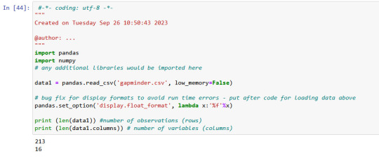
There is 213 rows ans 16 columns in gapminder data, which I used.

Displaying of selected variables (country, breastcanserper100th and Co2emissions) as a pandas dataframe.

Value 'breastcanserper100th'

Here I used .describe() command to see important statistical values

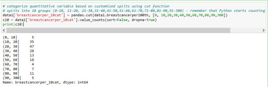
total 213 countries

but we have only 173 rows for breastcanserper100th information rows.

it means there are some informations (40 rows for countries) not available.

mean value of breastcanserper100th is 37,4

max value is 101,1 per 100000 womens

min value is 3,9 per 100000 womens

distribution of breastcanserper100th is below in 10 groups

Value 'co2emissions'

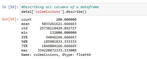
Information about co2emissions in using .describe() command for statistic

There is 200 values available

min co2emission value is 132000metric tons and max 334220872333.. metric tons

This is a very big difference.

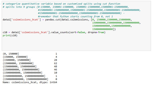
distribution of co2emissions is below in 9 groups

value 'lifeexpectancy

value 'lifeexpectancy' is for my subset data interesting. I converted it to numeric format and used describe() command to see statistic informations like mean and count. total 191 values available.

mean 69.75 years

max,83.39

min is 47,79

distribution of 'lifeexpectancy' is below in 10 groups

--------------------------------------------------------------------------

I think i have to check the cases , where the life expectancy< 69 and Co2 > 150000000 metric tons

which effects I can find out for breastcanserper100th

What is the distribution of breast cancer in different cases of lifeexpectancy and Co2 emissions?

it will be my next step.

[codewithnazam]

Data Manipulation: A Beginner's Guide to Pandas Dataframe Operations

Outline: What’s a Pandas Dataframe? (Think Spreadsheet on Steroids!) Say Goodbye to Messy Data: Pandas Tames the Beast Rows, Columns, and More: Navigating the Dataframe Landscape Mastering the Magic: Essential Dataframe Operations Selection Superpower: Picking the Data You Need Grab Specific Columns: Like Picking Out Your Favorite Colors Filter Rows with Precision: Finding Just the Right…

[machinelearningcoursera]

Lasso Regression

SCRIPT:

from pandas import Series, DataFrame import pandas as pd import numpy as np import os

from pandas import Series, DataFrame

import pandas as pd import numpy as np import matplotlib.pylab as plt from sklearn.model_selection import train_test_split from sklearn.linear_model import LassoLarsCV

Load the dataset

data = pd.read_csv("_358bd6a81b9045d95c894acf255c696a_nesarc_pds.csv") data=pd.DataFrame(data) data = data.replace(r'^\s*$', 101, regex=True)

upper-case all DataFrame column names

data.columns = map(str.upper, data.columns)

Data Management

data_clean = data.dropna()

select predictor variables and target variable as separate data sets

predvar= data_clean[['SEX','S1Q1E','S1Q7A9','S1Q7A10','S2AQ5A','S2AQ1','S2BQ1A20','S2CQ1','S2CQ2A10']]

target = data_clean.S2AQ5B

standardize predictors to have mean=0 and sd=1

predictors=predvar.copy() from sklearn import preprocessing predictors['SEX']=preprocessing.scale(predictors['SEX'].astype('float64')) predictors['S1Q1E']=preprocessing.scale(predictors['S1Q1E'].astype('float64')) predictors['S1Q7A9']=preprocessing.scale(predictors['S1Q7A9'].astype('float64')) predictors['S1Q7A10']=preprocessing.scale(predictors['S1Q7A10'].astype('float64')) predictors['S2AQ5A']=preprocessing.scale(predictors['S2AQ5A'].astype('float64')) predictors['S2AQ1']=preprocessing.scale(predictors['S2AQ1'].astype('float64')) predictors['S2BQ1A20']=preprocessing.scale(predictors['S2BQ1A20'].astype('float64')) predictors['S2CQ1']=preprocessing.scale(predictors['S2CQ1'].astype('float64')) predictors['S2CQ2A10']=preprocessing.scale(predictors['S2CQ2A10'].astype('float64'))

split data into train and test sets

pred_train, pred_test, tar_train, tar_test = train_test_split(predictors, target, test_size=.3, random_state=150)

specify the lasso regression model

model=LassoLarsCV(cv=10, precompute=False).fit(pred_train,tar_train)

print variable names and regression coefficients

dict(zip(predictors.columns, model.coef_))

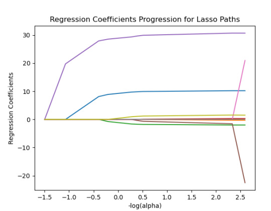
plot coefficient progression

m_log_alphas = -np.log10(model.alphas_) ax = plt.gca() plt.plot(m_log_alphas, model.coef_path_.T) plt.axvline(-np.log10(model.alpha_), linestyle='--', color='k', label='alpha CV') plt.ylabel('Regression Coefficients') plt.xlabel('-log(alpha)') plt.title('Regression Coefficients Progression for Lasso Paths')

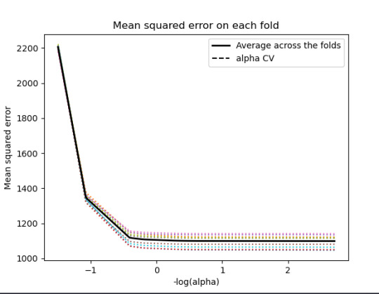
plot mean square error for each fold

m_log_alphascv = -np.log10(model.cv_alphas_) plt.figure() plt.plot(m_log_alphascv, model.mse_path_, ':') plt.plot(m_log_alphascv, model.mse_path_.mean(axis=-1), 'k', label='Average across the folds', linewidth=2) plt.axvline(-np.log10(model.alpha_), linestyle='--', color='k', label='alpha CV') plt.legend() plt.xlabel('-log(alpha)') plt.ylabel('Mean squared error') plt.title('Mean squared error on each fold')

MSE from training and test data

from sklearn.metrics import mean_squared_error train_error = mean_squared_error(tar_train, model.predict(pred_train)) test_error = mean_squared_error(tar_test, model.predict(pred_test)) print ('training data MSE') print(train_error) print ('test data MSE') print(test_error)

R-square from training and test data

rsquared_train=model.score(pred_train,tar_train) rsquared_test=model.score(pred_test,tar_test) print ('training data R-square') print(rsquared_train) print ('test data R-square') print(rsquared_test)

------------------------------------------------------------------------------

Graphs:

------------------------------------------------------------------------------

Analysing:

Output:

{'SEX': 10.217613940138108, 'S1Q1E': -0.31812083770240274, -ORIGIN OR DESCENT 'S1Q7A9': -1.9895640844032882, -PRESENT SITUATION INCLUDES RETIRED 'S1Q7A10': 0.30762235836398083, -PRESENT SITUATION INCLUDES IN SCHOOL FULL TIME 'S2AQ5A': 30.66524941440075, 'S2AQ1': -41.766164381325154, -DRANK AT LEAST 1 ALCOHOLIC DRINK IN LIFE 'S2BQ1A20': 73.94927622433774, - EVER HAVE JOB OR SCHOOL TROUBLES BECAUSE OF DRINKING 'S2CQ1': -33.74074926708572, -EVER SOUGHT HELP BECAUSE OF DRINKING 'S2CQ2A10': 1.6103002338271737} -EVER WENT TO EMPLOYEE ASSISTANCE PROGRAM (EAP)

training data MSE 1097.5883983117358 test data MSE 1098.0847471196266 training data R-square 0.50244242170729 test data R-square 0.4974333966086808

------------------------------------------------------------------------------

Conclusions:

I was looking at the questions, how often Brank beer in the last 12 Months?

We can see that the following variables are the most important variables to be able to answer the questions.

S2BQ1A20:EVER HAVE JOB OR SCHOOL TROUBLES BECAUSE OF DRINKING

S2AQ1:DRANK AT LEAST 1 ALCOHOLIC DRINK IN LIFE

S2CQ1:EVER SOUGHT HELP BECAUSE OF DRINKING

All the important variables are related to drinking. The Root squared for both the training and the test data is very small and very similar which means the training data set wasn't overfitted and not too biased.

30% was the training set and 70% was the test set, each set had 150 random states. The graph are showing 10 lasso regression coefficients

[rbem-amo]

Data analysis Tools: Module 3. Pearson correlation coefficient (r / r2)

According my last studies ( ANOVA and Chi square test of independence), there is a relationship between the variables under observation:

Quantitative variable: Femaeemployrate (Percentage of female population, age above 15, that has been employed during the given year)

Quantitative variable: Incomeperperson (Gross Domestic Product per capita in constant 2000 US$).

I have calculated the Pearson Correlation coefficient and I have created the graphic:

“association between Income per person and Female employ rate

PearsonRResult(statistic=0.3212540576761761, pvalue=0.015769942076727345)”

r=0.3212540576761761à It means that the correlation between female employ rate and income per person rate is positive and it is stark (near to 0)

p-value=0,015 < 0.05 it means that the is a relationship

The graphic shows the positive correlation.

In the graphic in the low range of the x axis is obserbed a different correlation, perhaps this correlation should be also analysis.

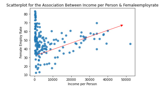
And the r2=0,32125*0,32125= 0,10

It can be predicted 10% of the variability in the rate of female employ rate according the income per person. (The fraction of the variability of one variable that can be predicted by the other).

Program:

# -*- coding: utf-8 -*-

"""

Created on Thu Aug 31 13:59:25 2023

@author: ANA4MD

"""

import pandas

import numpy

import seaborn

import scipy

import matplotlib.pyplot as plt

data = pandas.read_csv('gapminder.csv', low_memory=False)

# lower-case all DataFrame column names - place after code for loading data above

data.columns = list(map(str.lower, data.columns))

# bug fix for display formats to avoid run time errors - put after code for loading data above

pandas.set_option('display.float_format', lambda x: '%f' % x)

# to fix empty data to avoid errors

data = data.replace(r'^\s*$', numpy.NaN, regex=True)

# checking the format of my variables and set to numeric

data['femaleemployrate'].dtype

data['polityscore'].dtype

data['incomeperperson'].dtype

data['urbanrate'].dtype

data['femaleemployrate'] = pandas.to_numeric(data['femaleemployrate'], errors='coerce', downcast=None)

data['polityscore'] = pandas.to_numeric(data['polityscore'], errors='coerce', downcast=None)

data['incomeperperson'] = pandas.to_numeric(data['incomeperperson'], errors='coerce', downcast=None)

data['urbanrate'] = pandas.to_numeric(data['urbanrate'], errors='coerce', downcast=None)

data['incomeperperson']=data['incomeperperson'].replace(' ', numpy.nan)

# to create bivariate graph for the selected variables

print('relationship femaleemployrate & income per person')

# bivariate bar graph Q->Q

scat2 = seaborn.regplot(

    x="incomeperperson", y="femaleemployrate", fit_reg=False, data=data)

plt.xlabel('Income per Person')

plt.ylabel('Female Employ Rate')

plt.title('Scatterplot for the Association Between Income per Person & Femaleemployrate')

data_clean=data.dropna()

print ('association between Income per person and Female employ rate')

print (scipy.stats.pearsonr(data_clean['incomeperperson'], data_clean['femaleemployrate']))

Results:

relationship femaleemployrate & income per person

association between Income per person and Female employ rate

PearsonRResult(statistic=0.3212540576761761, pvalue=0.015769942076727345)

Data analysis Tools: Module 3. Pearson correlation coefficient (r / r2)

According my last studies ( ANOVA and Chi square test of independence), there is a relationship between the variables under observation:

Quantitative variable: Femaeemployrate (Percentage of female population, age above 15, that has been employed during the given year)

Quantitative variable: Incomeperperson (Gross Domestic Product per capita in constant 2000 US$).

I have calculated the Pearson Correlation coefficient and I have created the graphic:

“association between Income per person and Female employ rate

PearsonRResult(statistic=0.3212540576761761, pvalue=0.015769942076727345)”

r=0.3212540576761761à It means that the correlation is positive and it is stark (near to 0)

p-value=0,015 < 0.05 à it means that the is a relationship

The graphic shows the positive correlation.

And the r2=0,32125*0,32125= 0,10àwe can predict 10% of the variability in the rate of female employ rate according the income per person. (The fraction of the variability of one variable that can be predicted by the other).

Program:

# -*- coding: utf-8 -*-

"""

Created on Thu Aug 31 13:59:25 2023

@author: ANA4MD

"""

import pandas

import numpy

import seaborn

import scipy

import matplotlib.pyplot as plt

data = pandas.read_csv('gapminder.csv', low_memory=False)

# lower-case all DataFrame column names - place after code for loading data above

data.columns = list(map(str.lower, data.columns))

# bug fix for display formats to avoid run time errors - put after code for loading data above

pandas.set_option('display.float_format', lambda x: '%f' % x)

# to fix empty data to avoid errors

data = data.replace(r'^\s*$', numpy.NaN, regex=True)

# checking the format of my variables and set to numeric

data['femaleemployrate'].dtype

data['polityscore'].dtype

data['incomeperperson'].dtype

data['urbanrate'].dtype

data['femaleemployrate'] = pandas.to_numeric(data['femaleemployrate'], errors='coerce', downcast=None)

data['polityscore'] = pandas.to_numeric(data['polityscore'], errors='coerce', downcast=None)

data['incomeperperson'] = pandas.to_numeric(data['incomeperperson'], errors='coerce', downcast=None)

data['urbanrate'] = pandas.to_numeric(data['urbanrate'], errors='coerce', downcast=None)

data['incomeperperson']=data['incomeperperson'].replace(' ', numpy.nan)

# to create bivariate graph for the selected variables

print('relationship femaleemployrate & income per person')

# bivariate bar graph Q->Q

scat2 = seaborn.regplot(

    x="incomeperperson", y="femaleemployrate", fit_reg=False, data=data)

plt.xlabel('Income per Person')

plt.ylabel('Female Employ Rate')

plt.title('Scatterplot for the Association Between Income per Person & Femaleemployrate')

data_clean=data.dropna()

print ('association between Income per person and Female employ rate')

print (scipy.stats.pearsonr(data_clean['incomeperperson'], data_clean['femaleemployrate']))

Results:

relationship femaleemployrate & income per person

association between Income per person and Female employ rate

PearsonRResult(statistic=0.3212540576761761, pvalue=0.015769942076727345)

[courserabamarshall]

rom pandas import Series, DataFrame import pandas as pd import numpy as np import matplotlib.pylab as plt from sklearn.model_selection import train_test_split from sklearn import preprocessing from sklearn.cluster import KMeans

""" Data Management """ data = pd.read_csv("tree_addhealth")

upper-case all DataFrame column names

data.columns = map(str.upper, data.columns)

Data Management

data_clean = data.dropna()

subset clustering variables

cluster=data_clean[['ALCEVR1','MAREVER1','ALCPROBS1','DEVIANT1','VIOL1', 'DEP1','ESTEEM1','SCHCONN1','PARACTV', 'PARPRES','FAMCONCT']] cluster.describe()

standardize clustering variables to have mean=0 and sd=1

clustervar=cluster.copy() clustervar['ALCEVR1']=preprocessing.scale(clustervar['ALCEVR1'].astype('float64')) clustervar['ALCPROBS1']=preprocessing.scale(clustervar['ALCPROBS1'].astype('float64')) clustervar['MAREVER1']=preprocessing.scale(clustervar['MAREVER1'].astype('float64')) clustervar['DEP1']=preprocessing.scale(clustervar['DEP1'].astype('float64')) clustervar['ESTEEM1']=preprocessing.scale(clustervar['ESTEEM1'].astype('float64')) clustervar['VIOL1']=preprocessing.scale(clustervar['VIOL1'].astype('float64')) clustervar['DEVIANT1']=preprocessing.scale(clustervar['DEVIANT1'].astype('float64')) clustervar['FAMCONCT']=preprocessing.scale(clustervar['FAMCONCT'].astype('float64')) clustervar['SCHCONN1']=preprocessing.scale(clustervar['SCHCONN1'].astype('float64')) clustervar['PARACTV']=preprocessing.scale(clustervar['PARACTV'].astype('float64')) clustervar['PARPRES']=preprocessing.scale(clustervar['PARPRES'].astype('float64'))

split data into train and test sets

clus_train, clus_test = train_test_split(clustervar, test_size=.3, random_state=123)

k-means cluster analysis for 1-9 clusters

from scipy.spatial.distance import cdist clusters=range(1,10) meandist=[]

for k in clusters: model=KMeans(n_clusters=k) model.fit(clus_train) clusassign=model.predict(clus_train) meandist.append(sum(np.min(cdist(clus_train, model.cluster_centers_, 'euclidean'), axis=1)) / clus_train.shape[0])

""" Plot average distance from observations from the cluster centroid to use the Elbow Method to identify number of clusters to choose """

plt.plot(clusters, meandist) plt.xlabel('Number of clusters') plt.ylabel('Average distance') plt.title('Selecting k with the Elbow Method')

Interpret 3 cluster solution

model3=KMeans(n_clusters=3) model3.fit(clus_train) clusassign=model3.predict(clus_train)

plot clusters

from sklearn.decomposition import PCA pca_2 = PCA(2) plot_columns = pca_2.fit_transform(clus_train) plt.scatter(x=plot_columns[:,0], y=plot_columns[:,1], c=model3.labels_,) plt.xlabel('Canonical variable 1') plt.ylabel('Canonical variable 2') plt.title('Scatterplot of Canonical Variables for 3 Clusters') plt.show()

""" BEGIN multiple steps to merge cluster assignment with clustering variables to examine cluster variable means by cluster """

create a unique identifier variable from the index for the

cluster training data to merge with the cluster assignment variable

clus_train.reset_index(level=0, inplace=True)

create a list that has the new index variable

cluslist=list(clus_train['index'])

create a list of cluster assignments

labels=list(model3.labels_)

combine index variable list with cluster assignment list into a dictionary

newlist=dict(zip(cluslist, labels)) newlist

convert newlist dictionary to a dataframe

newclus=DataFrame.from_dict(newlist, orient='index') newclus

rename the cluster assignment column

newclus.columns = ['cluster']

now do the same for the cluster assignment variable

create a unique identifier variable from the index for the

cluster assignment dataframe

to merge with cluster training data

newclus.reset_index(level=0, inplace=True)

merge the cluster assignment dataframe with the cluster training variable dataframe

by the index variable

merged_train=pd.merge(clus_train, newclus, on='index') merged_train.head(n=100)

cluster frequencies

merged_train.cluster.value_counts()

""" END multiple steps to merge cluster assignment with clustering variables to examine cluster variable means by cluster """

FINALLY calculate clustering variable means by cluster

clustergrp = merged_train.groupby('cluster').mean() print ("Clustering variable means by cluster") print(clustergrp)

validate clusters in training data by examining cluster differences in GPA using ANOVA

first have to merge GPA with clustering variables and cluster assignment data

gpa_data=data_clean['GPA1']

split GPA data into train and test sets

gpa_train, gpa_test = train_test_split(gpa_data, test_size=.3, random_state=123) gpa_train1=pd.DataFrame(gpa_train) gpa_train1.reset_index(level=0, inplace=True) merged_train_all=pd.merge(gpa_train1, merged_train, on='index') sub1 = merged_train_all[['GPA1', 'cluster']].dropna()

import statsmodels.formula.api as smf import statsmodels.stats.multicomp as multi

gpamod = smf.ols(formula='GPA1 ~ C(cluster)', data=sub1).fit() print (gpamod.summary())

print ('means for GPA by cluster') m1= sub1.groupby('cluster').mean() print (m1)

print ('standard deviations for GPA by cluster') m2= sub1.groupby('cluster').std() print (m2)

mc1 = multi.MultiComparison(sub1['GPA1'], sub1['cluster']) res1 = mc1.tukeyhsd() print(res1.summary())